10. Green’s Functions#
The coverage of Green’s functions in [Arfken et al., 2013] is quite reasonable. Here are some highlights presented from a different perspective, analogous to that in [Hassani, 2013]. I highly recommend comparing these two approaches – learning to translate from vectors and matrices to differential equations is an extremely valuable skill.
The general idea is to find particular solutions to a linear differential equation. Recall that this is a functional equivalent of solving a linear system:
Green’s functions are the functional equivalent of inverting \(\mat{L}\):
\(G(x,y) = G(x-y)\) as a Toeplitz matrix.
Green’s functions are often presented in the form
which obscures the matrix nature of \(G\). This can be done when \(\mathcal{L}\) is independent of \(x\) – i.e., translationally invariant. In this case
This corresponds to a Toeplitz matrix or diagonal-constant matrix \(\mat{G}\) where the entries depend only on their distance from the diagonal. I.e. the diagonal has one constant value, the next diagonal has another constant value etc.
Toeplitz matrices have many nice properties, including the fact that they are diagonalized by plane waves
This is why Fourier techniques are so useful for finding Green’s functions.
Do It! Show that \(\mat{G}\ket{f_m} = \ket{f_m}\lambda_m\) if \(\mat{G}\) is a Toeplitz matrix.
(Incomplete)
While this often simplifies things, it is best to keep in mind the nature of Green’s functions as matrices, not as vectors.
Do It! Damped Harmonic Oscillator \(\mathcal{L}=\partial_{tt}+2\beta\partial_{t}+\omega_0^2\).
Find the general Green’s function for the damped harmonic oscillator. Recall that \(\mathcal{L}\) is independent of time (invariant under shifts of time), so we can write \(G(t, \tau) = G(t-\tau)\), thus find the general homogeneous solutions \(h_1(t)\) and \(h_2(t)\) such that
Note that there are many such solutions since \(G(t) + h(t)\) is also a valid Green’s function. Find the causal Green’s function where \(G_{+}(t < 0) = 0\).
Solution
Here we solve the slightly simpler case without damping where \(\beta = 0\). The homogeneous solutions are simply \(e^{\pm \I \omega_0 t}\) so we have
\(G(t)\) must be continuous at \(t=0\), so \(a_+ + a_- = b_+ + b_-\). Likewise, the derivatives must be discontinuous with a unit step so that we obtain \(\delta(t)\):
We can express these conditions as \(\braket{D_0|A} = 0\) and \(\braket{D_1|A} = 1\) in terms of the following vectors
Noting that
we can write the solution as
where \(\ket{B}\) is any vector orthogonal to the subspace \(\{\ket{D}_0, \ket{D}_1\}\). This subspace is easily constructed by inspection, but could be found using the Gram-Schmidt procedure (QR decomposition):
To find the causal Green’s function, we want \(a_+ = a_- = 0\). This requires \(b_+ = -b_- = b\) and then \(2\I \omega_0 b = 1\)
The full solution can be found most simply using Fourier techniques and contour integrals as follows. Express
Then, taking the Fourier transform of \(\mathcal{L}G = \delta\) gives
The Green’s function can be computed by a contour integral
where the contour is closed along a circular arc going to infinity. To ensure that the additional contributions vanish (justifying the last equality), we must close the contour up if \(t > 0\) and down if \(t<0\) to ensure that the exponential factor decays (see Jordan’s lemma).
If \(0 < \beta\), then both poles like in the upper half plane, so the integral is zero if \(t<0\) and the sum of both residues if \(t>0\):
which approaches our previous solution as \(\beta \rightarrow 0\).
If we strictly have \(\beta = 0\), then the two poles like on the real axis. In this case, we must choose how we go around them. There are four choices here: going below both gives the causal (retarded) Green’s function as above. Going over both gives the acausal (advanced) Green’s function that is zero for \(t>0\). Going over one and under the gives a Green’s function that is non-zero for all times. These mixed forms are often better suited for perturbation theory and play a key role in computing Feynman diagrams.
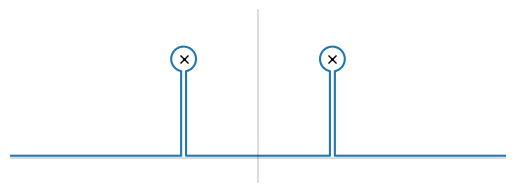
Does the previous calculation mean that there is only one Green’s function if \(\beta > 0\)? No: there are always others we can find by suitably deforming the contour as shown on the right.
Although formally \(\mat{G} = \mat{L}^{-1}\), the formalism presented this way works even if \(\mat{L}\) is singular. In particular, we are generally faced with a problem where \(\mathcal{L} h(x) = 0\) has homogeneous solutions.
Self-Adjoint Operators#
We now explain [Arfken et al., 2013] Eq. (10.18) (recast slightly):
for a second-order self-adjoint operator \(\mathcal{L}\) where \(h_1(x)\) is the homogeneous solution satisfying the left boundary condition and \(h_2(x)\) is a homogeneous solution satisfying the right boundary condition. The argument is simply that for \(x \neq y\), the functional dependence on \(x\) must be a homogeneous solution satisfying the boundary conditions, and \(\mat{G} = \mat{G}^\dagger\) hence \(G(x, y) = G(y, x)^*\). (The form here assumes that \(h_{i}\) are real.)
The constant \(A\) is found by ensuring that the discontinuity at \(x=y\) gives the delta-function. Note that in your solution for the causal Green’s function \(G_+(t)\) fo the Harmonic oscillator above, one cannot express \(G(t, \tau) = G_{+}(t-\tau) = \Theta(t-\tau)\sin\bigl(\omega_0(t-\tau)\bigr)/\omega_0\) in this form: this lack of symmetry is because the operator \(\mathcal{L}\) is not self-adjoint with the specified boundary conditions.
Details
This follows from the following arguments, made in terms of linear algebra but tagged with the corresponding equation in [Arfken et al., 2013]. We start with the definition of the Green’s function:
Since \(\mat{L}\) is Hermitian, it has a complete set of orthonormal eigenstates
This means we can express both \(\mat{G}\) and \(\mat{1}\) in the basis
Inserting these into (10.6) we have
Compute the matrix elements of this expression \(\braket{n|\cdots|m}\) (rename the inner dummy indices while you do this) to find (no summation convention)
Thus, we see that \(\mat{G}\) is also Hermitian.