Renormalizing Random Walks

Renormalizing Random Walks#

$\newcommand{\N}{\mathcal{N}}$ Here we work through the example discussed in [Creswick et al., 1992] and [McGreevy, 2018] about random walks.

Gaussian Random Walks: A Fixed Point#

Consider a gaussian random walk where each step is drawn from a normal distribution with “spherical” symmetry:

\[\begin{gather*} \vect{r}_n \sim \N(\vect{0}, \sigma^2\mat{1}), \qquad \end{gather*}\]

Here we demonstrate numerically in $d=2$ dimensions with $\sigma=1$:

../_images/f1e3050821b65ead23886e7cc79ceaa4b61372f6168ab4aff24c3aedc722c1d2.png

A Crash Course in Random Variables

We use the following notation for a random variable $\vect{x}$, which is said to take values from a distribution $\mathcal{P}$, whose probability density function (PDF) is $p_{\mathcal{P}}(\vect{x})$:

\[\begin{gather*} \DeclareMathOperator{\Pr}{Pr} \vect{x} \sim \mathcal{P}, \qquad \Pr(\vect{x}\in S) = \int_{\vect{x}\in S}\d^{d}{\vect{x}}\; p_{\mathcal{P}}(\vect{x}). \end{gather*}\]

For example, if $\vect{x}$ takes values from a multivariate normal distribution $\N(\vect{\mu}, \mat{\Sigma})$ with mean $\vect{\mu}$ and covariance matrix $\mat{\Sigma}$:

\[\begin{gather*} \vect{x} \sim \N(\vect{\mu}, \mat{\Sigma}), \qquad p(\vect{x}) = \frac{\exp\left( -\frac{1}{2}(\vect{x} - \vect{\mu})^T \mat{\Sigma}^{-1} (\vect{x} - \vect{\mu}) \right)} {\sqrt{\det|2\pi \mat{\Sigma}|}}. \end{gather*}\]

If one forms a new random variable $\vect{y} = \vect{f}(\vect{x})$, the PDF for $\vect{y}$ can be found by integrating with an appropriate delta function:

\[\begin{gather*} p_{y}(\vect{y}) = \int \d^{d}{\vect{x}}\; p_{x}(\vect{x})\delta^{d}(\vect{y} - \vect{f}(\vect{x})). \end{gather*}\]

Exercise

Show that the PDF of a sum of two independently distributed random variables is the [convolution] of the two independent PDFs,

\[\begin{gather*} p_{\vect{A} + \vect{B}}(\vect{x}) = (p_{\vect{A}} * p_{\vect{B}})(\vect{x}), \end{gather*}\]

and that, consequently, the sum of two normally distributed variables has the following

\[\begin{gather*} \vect{A}\sim\N(\vect{a}, \mat{\Sigma}_{a}), \qquad \vect{B}\sim\N(\vect{b}, \mat{\Sigma}_{b}), \\ \vect{X} = \vect{A} + \vect{B} \sim \N(\vect{a} + \vect{b}, \mat{\Sigma}_{a} + \mat{\Sigma}_{b}). \end{gather*}\]

I.e., the new distribution has just the sum of the means, and the sum of the covariance matrices.

(Note: The distributions must be independent, or at least jointly normal, otherwise the resulting distribution might not be a multivariate normal distribution.)

Now consider a 1-dimensional PDF $p(x)$ and its Fourier transform

\[\begin{gather*} \tilde{p}(k) = \braket{e^{-\I k x}} = \int_{-\infty}^{\infty} e^{-\I kx} p(x) \d{x}. \end{gather*}\]

Negating the argument, this is called the characteristic function $\varphi(t) = \tilde{p}(-t)$, and Wick rotating, this becomes the moment-generating function $g(t) = \tilde{p}(-\I t)$ and its logarithm $h(t):

\[\begin{align*} \tilde{p}(k) &= \braket{e^{-\I k x}},\\ \varphi(t) &= \tilde{p}(-t) = \braket{e^{\I t x}},\\ g(t) &= \tilde{p}(\I t) = \braket{e^{t x}},\\ h(t) &= \ln \tilde{p}(\I t) = \ln \braket{e^{t x}}. \end{align*}\]

Note that unlike the others, $g(t)$ and $h(t)$ need not be well defined, as is the case with heavy-tailed distributions like the Cauchy distribution.

The moment-generating function and its logarithm $h(t) = \ln g(t)$ are particularly useful for generating the moments $m_n$ and cumulants $C_n$ of the distribution as their derivatives (hence the name “generating function”)

\[\begin{align*} m_n &= \braket{x^n} = \left.\diff[n]{g(t)}{t}\right|_{t=0} = g^{(n)}(0),\\ C_n &= \left.\diff[n]{h(t)}{t}\right|_{t=0} = h^{(n)}(0). \end{align*}\]

The cumulants $C_n$ will be particularly useful here, and are the coefficients of the log of the Fourier transform:

\[\begin{gather*} \ln \tilde{p}(k) = C_0 - C_1 \I k - C_2 \frac{k^2}{2} + \cdots + C_n\frac{(-\I k)^n}{n!}+\cdots. \end{gather*}\]

Exercise: Moments $m_n$ and Cumulants $C_n$

Show that the first few moments and cumulants are defined in terms of the normalization, mean $\mu$ and standard deviation $\sigma$ of the distribution $p(x)$:

\[\begin{align*} m_0 &= 1, & m_1 &= \mu, & m_2 &= \mu^2 + \sigma^2,\\ C_0 &= 0, & C_1 &= \mu, & C_2 &= \sigma^2. \end{align*}\]

Show that $m_n = g^{(n)}(0)$ and $C_n = h^{(n)}(0)$ are indeed generated by $g(t) = \braket{e^{tx}}$ and $h(t) = \log g(t)$.

Show that the second and three cumulants $C_2$ and $C_3$ are the central moments, but that this pattern does not hold for the forth cumulant $C_4$:

\[\begin{align*} C_2 &= \braket{(x-\mu)^2} = \sigma^2 = m_2 - m_1^2,\\ C_3 &= \braket{(x-\mu)^3} = m_3 - 3m_2m_1 + 2 m_1^3,\\ C_4 &= \braket{(x-\mu)^4} - 3\sigma^4. % = m_4 - 4 m_3 m_1 + 12 m_2 m_1^2 - 3m_2^2- 6 m_1^4. \end{align*}\]

Exercise

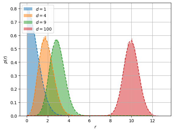
By “spherically” symmetric distribution (in $d$-dimensions) we mean that all directions are equally likely. Compute the probability density function of $p(r)$ of the radius $r = \norm{\vect{r}}_2$. Check your results against the following numerical implementation.

\[\begin{gather*} p(r) = \frac{1}{\sqrt{(2\pi \sigma)^d}}\int \d^{d}{\vect{x}}\; e^{-\norm{\vect{x}}_2^2/2\sigma^2}\delta(r-\norm{\vect{x}}_2)\\ = \frac{S_{d-1}}{\sqrt{(2\pi \sigma)^d}}r^{d-1}e^{-r^2/2\sigma^2}, \qquad S_{d-1} = \frac{2\pi^{d/2}}{\Gamma(\tfrac{d}{2})} \end{gather*}\]

where $S_{d-1}$ is the volume of a unit $d$-dimensional sphere.

# Define a random number generator with a seed so the results are reproducible
from scipy.special import gamma
rng = np.random.default_rng(seed=2)

fig, ax = plt.subplots()
dims = [1, 4, 9, 100]
Nsamples = 100000
r_ = np.linspace(0, 12)
for n, d in enumerate(dims):
    r = np.linalg.norm(rng.normal(size=(Nsamples, d)), axis=-1)
    ax.hist(r, bins=100, label=f"$d={d}$", color=f"C{n}",
            histtype='stepfilled', density=True, alpha=0.5)
    fact = 2*np.pi**(d/2)/gamma(d/2) / np.sqrt(2*np.pi)**d
    ax.plot(r_, fact * r_**(d-1)*np.exp(-r_**2/2), f"--C{n}")
ax.set(xlabel="$r$", ylabel="$p(r)$")
ax.grid('on')
ax.legend(loc="upper left");

../_images/537ae715e0f7c2a8f147d8362b8eac9e1ea731b560e54b8b565c1ad9c358f6cd.png

The first step of RG is to coarse grain. In this context, we might consider taking $N$ steps at a time:

\[\begin{align*} \vect{R}_{0} &= \vect{r}_{0} + \vect{r}_{1} + \dots + \vect{r}_{N-1},\\ \vect{R}_{1} &= \vect{r}_{N} + \vect{r}_{N+1} + \dots + \vect{r}_{2N-1},\\ & \vdots \end{align*}\]

Show from the properties of random variables that

\[\begin{gather*} \vect{R}_{n} \sim \N(\vect{0}, N\sigma^2 \mat{1}), \end{gather*}\]

Thus, if we rescale our distance by a factor of $\sqrt{N}$, we obtain the same distribution:

\[\begin{gather*} \frac{\vect{R}_{n}}{\sqrt{N}} \sim \N(\vect{0}, \sigma^2 \mat{1}). \end{gather*}\]

This is an example of an RG fixed point.

Examples#

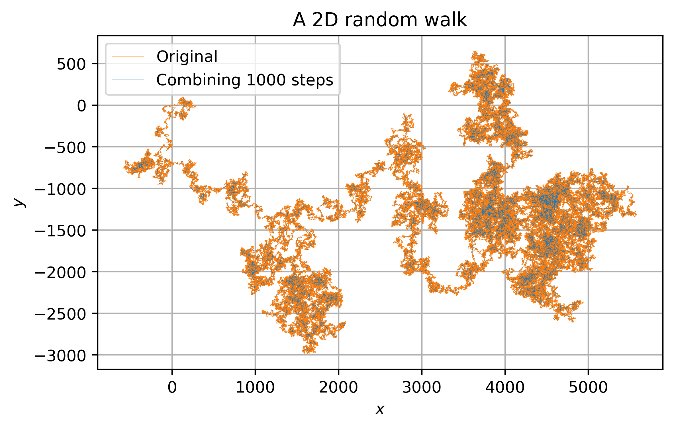
Here we show a 2D unbiased random walk with $\sigma = 1$ rescaled as discussed above by $\lambda = 1/\sqrt{N}$. The picture of the full RG flow is as follows:

Coarse-graining/Changing Scale: Physically, we step back and look at the random walk from “further away”, so we can no-longer resolve details on the original scale. We now “see” every $N$ steps as a single step because our “eyes cannot” resolve the smaller detail. In the figure below, the original region on the left shrinks when we do this to the small box in the right.

Rescaling: We now try to scale the variables in our theory so that the results “look” like they did before. In this case, we should take the same number of steps, and then try to adjust the units so that the random walk wanders the same distance away from the starting point. The following figure shows that the scaling we specified above $\lambda = 1/\sqrt{N}$ works.

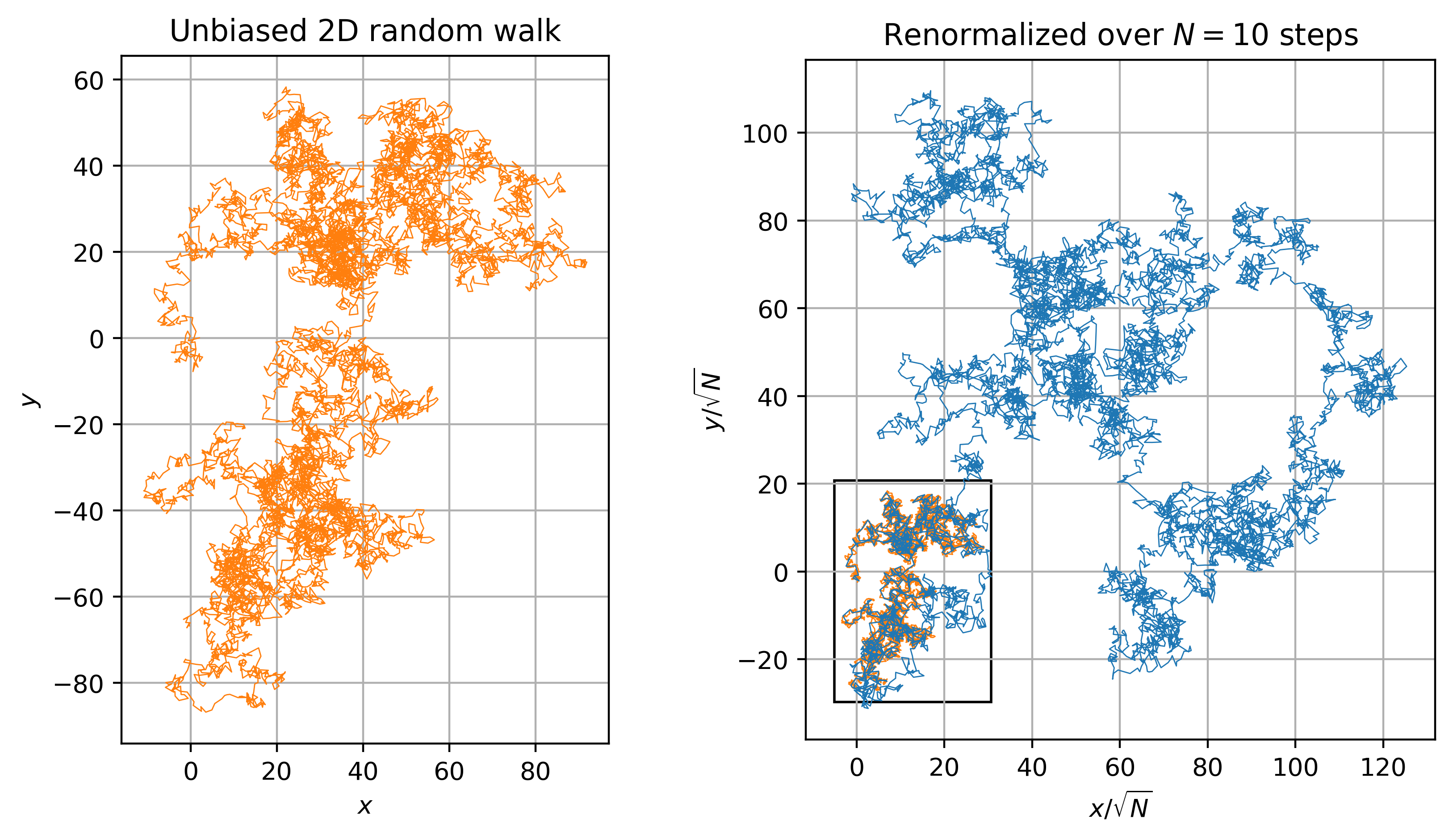
../_images/6b63b047510de618ee9851de210934bf46851f4f075b913b89061b37ce6aaaed.png

Notice that after effecting this RG transformation of taking $N$ steps then scaling by $\lambda = 1/\sqrt{N}$, we end up with a curve that has the same statistical properties as the original. (Since this is a random walk, the actual curve is different, but notice that the smoothness, extent of the walk, etc. are roughly the same.)

Random Walks: Universality#

What about if our random walk is not gaussian? Then, in general, the distribution of the coarse-grained steps $\vect{R}_n$ will not be related to those of $\vect{r}_{n}$ by a simple scaling. To analyze this behavior, we need a nice way of parameterizing the distributions. Recall that when we add random variables, the PDF is a convolution. Thus, it is natural to work with the Fourier transform of the distribution:

\[\begin{gather*} \tilde{p}(\vect{k}) = \int\d^{d}{\vect{r}}\; e^{-\I\vect{k}\cdot\vect{x}}p(\vect{r}),\qquad \tilde{p}_{R}(\vect{k}) \propto \Bigl(\tilde{p}(\vect{k})\Bigr)^{N},\\ p_{R}(\vect{R}) \propto \int \frac{\d^{d}{\vect{k}}}{(2\pi)^d}\; e^{\I \vect{R}\cdot\vect{k}}\Bigl(\tilde{p}(\vect{k})\Bigr)^{N}. \end{gather*}\]

For simplicity, consider a $d=1$-dimensional random walk. One way of parameterizing the distribution is to express the logarithm of $\tilde{p}(k)$ as power series:

\[\begin{gather*} \tilde{p}(k) = \exp\left( C_0 - C_1\I k - C_2\frac{k^2}{2} + \cdots + C_{n}\frac{(-\I k)^n}{n!} + \cdots \right),\\ \tilde{p}_{R}(k) \propto \exp\left( NC_0 - NC_1 \I k - NC_2\frac{k^2}{2} + \cdots + NC_{n}\frac{(-\I k)^n}{n!} + \cdots \right). \end{gather*}\]

As discussed above, these coefficients $C_n = h^{(n)}(0)$ are the cumulants, generated by the derivatives of $h(t) = \ln \braket{e^{tx}}$.

Now, if we perform the RG transformation, we must also rescale $k\rightarrow k/\sqrt{N}$, so under the full RG transformation, we have the flow:

\[\begin{gather*} \tilde{p}(k) \rightarrow \tilde{p}_{R}\left(\frac{k}{\sqrt{N}}\right)\\ \propto \exp\left(NC_0 - \sqrt{N} C_1 \I k - C_2\frac{k^2}{2} + \cdots + C_{n}\frac{(-\I k)^n}{N^{n/2}n!} + \cdots \right). \end{gather*}\]

In other words, the coefficients scale as

\[\begin{gather*} C_{n} \rightarrow N^{1-n/2}C_{n}. \end{gather*}\]

In RG parlance, the coefficients $C_0$ and $C_1$ are called relevant since they grow, the coefficient $C_2$ is called marginal since it does not grow, and the remaining coefficients $C_3$, $C_4$, etc. are called irrelevant since they get smaller.

Exercise

The parameter $C_0$ is not really a parameter, since it must be adjusted to preserve the normalization. Show that this implies $C_0 = 0$, which is consistent with the RG flow.

Symmetries#

This RG flow has some special properties: in particular, the coefficients $C_{n}$ do not mix under the flow. Technically, we have chosen a nice parameterization of our theory in terms of eigenvectors of the flow. In general this will not happen, and different coefficients will mix as we evolve the flow.

One important exception is if the theory has underlying symmetries. In this case, if we start the flow in a sector of the theory that respects a certain symmetry, then we expect that the flow will not generate terms that break the symmetry.

Anomalies

The existence of a formal “symmetry” is not a guarantee that RG flow will not generate terms that break the symmetry. In this case, the symmetry is said to be anomalously broken. This generally arises as follows:

When calculating, one encounters effects that need regularization, such as divergences. (See sec:RG-SEQ for a detailed discussion.) One finds that all ways of regularizing require introducing a parameter that breaks the symmetry. One hopes that, by taking the parameter to zero at the end of the calculation, the symmetry will be restored, but finds that the symmetry remains broken.

E.g. a theory might appear to be rotational invariant, but to calculate, one might discretize the theory by putting the theory on a cubic lattice which breaks rotations. As one takes the lattice spacing to zero – called the continuum limit – one expects rotational invariance to be restored. If it is not, rotation is said to be anomalously broken. A scale anomaly plays a crucial role in QCD, which is a dimensionless theory from which a physical mass unit emerges (~1GeV – the mass of a proton), a dissipative anomaly appears in [classical turbulence] breaking time-reversal, and a chiral anomaly plays a fundamental role in the [Standard Model] of particle physics.

The presence of anomalies is often associated with topological properties of the theory. Locally, the theory appears to have a symmetry, but the topology of the underlying space prevents the symmetry from being realized globally. Consider for example the hairy ball theorem: you can locally comb your hair flat, but you can’t do it everywhere on the entire sphere. (I am not sure if this is associated with any anomaly…)

In our previous example of an unbiased random walk, the probability distribution was symmetric under parity $x \rightarrow -x$ or $\vect{r} \rightarrow -\vect{r}$. This symmetry ensures¹ that if $C_1 = 0$, then it will remain zero, even though the operator is relevant under the RG transform.

Universality#

We thus arrive at the important result that a large class of initial probability distributions will flow towards RG fixed points $\vect{R}_n \sim \N(\vect{0}, \mat{\Sigma})$ with gaussian PDFs. If we restrict our consideration further to isotropic random (spherical symmetry) then these flow to a single fixed-point $\vect{R}_n \sim \N(\vect{0}, \mat{1})$ once appropriately scaled. This is part of the idea of universality: near the fixed-point, a whole class of complicated (many parameters $\{C_n\}$) microscopic theories flow towards a single simple theory characterized by the single parameter $C_2 = \sigma^2$ that can also be removed by setting an appropriate scale.

The idea of universality goes further: near this fixed point, the theory demonstrates a particular scaling which is the same for a large class of fixed points from possibly very different theories. Consider the root-mean-square (rms) distance $r_{\mathrm{rms}}(N)$ for a random walk of $N$ steps. By dimensional arguments, this must be proportional to $\sigma$ – the only dimensionful parameter in the theory at the isotropic fixed-point:

\[\begin{gather*} r_{\mathrm{rms}}(N) \sim \sigma N^\nu. \end{gather*}\]

The number of steps $N$ is dimensionless, so we cannot a-priori say anything about the value of the exponent $\nu$. The second idea of universality is that many theories all behave similarly near the critical point with the same value of the critical exponent $\nu$. Systems that behave with different exponents near the fixed-point are said to belong to different universality classes.

In our case here, we have shown that the RG fixed point for isotropic random walks is characterized by the invariance:

\[\begin{gather*} \frac{r_{\mathrm{rms}}(N)}{\sqrt{N}} \sim \sigma. \end{gather*}\]

Hence these are all in the same universality class with critical exponent $\nu = 1/2$. Note that this exponent does not depend on the dimension $d$: thus, not only do a whole set of isotropic microscopic random walks renormalized toward the same type of fixed-point (first universality concept), but many theories in different dimensions also belong to the same universality class (second universality concept).

Exercise

Calculate $r_{\mathrm{rms}}(N)$ explicitly and show that $\nu = 1/2$. Verify this numerically.

Biased Random Walk#

The rescaling part of RG always bothered me. Why is it not enough to just coarse graining? After all, coarse graining is how we get thermodynamics, hydrodynamics etc. Similarly, if we are going to rescale, how do we know how to choose the appropriate rescaling? It always seemed somewhat arbitrary.

Here we initially identified that the RG transformation of taking $N$ steps and then scaling by $1/\sqrt{N}$ led to a RG fixed point for gaussian distributions, but when we considered the full Fourier expansion:

\[\begin{gather*} \tilde{p}_{R}(k) \propto \exp\left( - NC_1 \I k - NC_2\frac{k^2}{2} + \cdots + NC_{n}\frac{(-\I k)^n}{n!} + \cdots \right) \end{gather*}\]

it seems like we could have chosen a different scaling, for example $k \rightarrow k/N$ which gives

\[\begin{gather*} \tilde{p}_{R}(k) \propto \exp\left( - C_1 \I k - C_2\frac{k^2}{2N} + \cdots + C_{n}\frac{(-\I k)^n}{N^{n-1}n!} + \cdots \right), \\ C_{n} \rightarrow N^{1-n}C_{n}. \end{gather*}\]

In this case, the coefficient $C_2$ is now irrelevant, and $C_1$ becomes marginal. This is also a valid RG procedure and also leads to an RG fixed point, but now in the case of a biased random walk.

The essential point is to choose a scaling so that RG transformation minimizes changes in the theory. Here we demonstrate what would have happened if we applied the previous RG analysis to a biased random walk, again with $\sigma = 1$ but now with a small bias to the upper right of $\vect{\mu} = (0.05, 0.05)$.

../_images/1159dbc6b753908fb788f76d1b8f43ebec42526e4423bc4f362a7c34ce0cc400.png

In the left plot, we see that the biased random walk drifts to the upper right, moving about 500 units right and 500 units up. I the middle plot, we take the same number of $N$ steps at a time, and try rescaling by $1/\sqrt{N}$ as before. This rescaling, however, does not preserve the qualitative structure of the walk, which now goes much further. Instead, we see that scaling by $1/N$ restores the qualitative behavior of drifting about 500 units. We also see that the fluctuations associated with the now-irrelevant $C_2 = \sigma^2$ parameter are getting smaller.

Dropping the restriction of isotropy, we now find a different universality class with $\nu = 1$:

\[\begin{gather*} r_{\mathrm{rms}}(N) \sim \sigma N^1. \end{gather*}\]

Basins of Attraction#

A alternative picture can be given in terms of the original RG flow with $1/\sqrt{N}$ rescaling. Consider the “space of theories” as the vector $\vect{C} = (C_1, C_2, \dots)$ of parameters. Under the original RG flow, $C_n \rightarrow N^{1-n/2}C_n$, we have one relevant parameter $C_1 \rightarrow \sqrt{N} C_1$ and one marginal parameter $C_2 \rightarrow C_2$: the rest are irrelevant.

The RG transformation can be thought of as flow in this space:

\[\begin{gather*} \diff{C_n}{N} = \frac{1-\tfrac{n}{2}}{N^{n/2}}C_n. \end{gather*}\]

No matter where we start $\vect{C}(0)$, the theory will “flow” towards the $(C_1, C_2)$ plane with all higher coefficients flowing to $\lim_{N\rightarrow \infty} C_{n>2}(N) = 0$. This plane is said to be an attractor, and this is the idea that complicated theories tend to flow towards simpler theories.

Now consider the flow in this plane (coarse graining with steps of $N=2$):

../_images/ebb10fddcd184a6c4c2f579137e8a586dd540c1941f78e0e46bed744a5dea04e.png

The left plot shows a slice through the attractive $(C_1, C_2)$ plane. Here we see a line of fixed points at $C_1=0$: if we start with parity, then we will remain on this line. However, if we start with even a small $C_1$, then eventually the flow will diverge to the second fixed point at $C_2 \rightarrow \infty$, which we identified above as a different universality class with $\nu = 1$.

The right plot shows a slice through the $(C_1, C_3)$ plane (ignoring the “boring” marginal parameter $C_2$). Here we see quite typical RG flow: the irrelevant parameter $C_3$ flows toward the fixed point, while the relevant parameter $C_1$ flows away. Consider the flow shown as the thick black line of a microscopic theory starting with $(C_1, C_2, C_3) = (0.001, 1.0, -1)$.

:tags: [hide]
from scipy.optimize import root

def f(a, C=(0.02, 1, 0.2), N=1000000):
    rng = np.random.default_rng(2)
    x = rng.normal(size=N)
    y = a[0]*x*np.cosh(a[1] + x)/(np.cosh(a[2] + x))
    C1 = y.mean()
    C2 = y.std()**2
    C3 = ((y-C1)**3).mean()
    Cs = np.asarray([C1, C2, C3])
    return Cs/C - 1


res = root(f, [1.0,-0.1,0])
print(res.x)
#rng = np.random.default_rng(2)
#a = res.x
#y = a[0]*x*np.cosh(x+a[1])/np.cosh(x+a[2])
#C1 = y.mean()
#C2 = y.std()**2
#assert np.allclose(C2, ((y-C1)**2).mean())
#C3 = ((y-C1)**3).mean()
#plt.hist(y, 100, density=True);
#C1, C2, C3, a

%matplotlib inline
from ipywidgets import interact, widgets
import numpy as np, matplotlib.pyplot as plt
# Here we generate a 1D random walk with a non-gausian "microscopic"
# probability, then coarse-grain and rescale to demonstrate how the
# distribution changes.

class RandomWalk:
    """View a 1D random walk from various scales."""
    # Parameters to generate transformation
    a = [0.92424594, 1.88032074, 1.75306592]
    a = [ 1.09839427, -2.1781062, -2.31120397]
    N = 2  # Coarse graining step number
    Nwalks = 5
    Nsamples = N**20
    Nsteps = N**10   # Each frame shows this many steps

    def __init__(self, **kw):
        for k in kw:
            if not hasatter(self, k):
                raise ValueError(f"Unknown parameter {k}")
            setattr(self, k, kw[k])
        self.init()
        
    def init(self):
        self.walks = self.get_walks()
        self.steps = np.arange(self.Nsamples)
        self.Nscales = int(np.log2(self.Nsamples // self.Nsteps)/np.log2(self.N))
        self.colors = [f"C{_n}" for _n in range(self.Nwalks)]
        
    def get_walks(self, seed=2):
        rng = np.random.default_rng(seed=seed)
        x = rng.normal(size=(self.Nwalks, self.Nsamples))
        # Change variables to a non-gaussian 
        a = self.a
        r = a[0]*x*np.cosh(x+a[1])/np.cosh(x+a[2])
        C1 = r.mean()
        C2 = r.std()**2
        C3 = ((r-C1)**3).mean()
        self.Cs = [C1, C2, C3]
        print(f"C1={C1:.4f}, C2={C2:.4f}, C3={C3:.4f}")
        walks = np.cumsum(r, axis=-1)
        return walks

    def draw_background(self, ax):
        for walk, color in zip(self.walks, self.colors):
            ax.plot(walk, self.steps, color)
    
    def get_frame(self, RG_step, ax, loc=0, data=data):
        """
        Argumets
        --------
        loc : float
            Location along total walk of zoom.
        """
        walks, steps = self.walks, self.steps
        ind = int(loc*(self.Nsamples-1))
        x0, y0 = walks[0, ind], steps[ind]
        C1, C2, C3 = self.Cs
        sigma = np.sqrt(C2)
        N = 2**RG_step
        dx = sigma * np.sqrt(N)
        lam = 1/np.sqrt(N)
        ax.set(xlim=(x0-10*dx, x0+10*dx),
               ylim=(ind-N*Nsteps/2, ind+N*Nsteps/2),
               title=f"C1={C1:.4f}, C2={C2:.4f}, C3={C3:.4f}")
        
        #x_, y_ = walks[:, ::N], steps[::N]
        #dx_ = np.diff(x_, axis=0)*lam
        #C1 = dx_.mean()
        #C2 = dx_.std()**2
        #C3 = ((dx_-C1)**3).mean()
        #for n in range(len(walks)):
        #    ax.plot(x_[n], y_, f"C{n}")
        #ax.set(xlim=(x_[:N].min(), x_[:N].max()), 
        #       ylim=(y_[:N].min(), y_[:N].max()),
        #       title=f"C1={C1:.4f}, C2={C2:.4f}, C3={C3:.4f}")

w = RandomWalk()
#fig, ax = plt.subplots()
#w.draw_background(ax)

@interact(loc=(0,1,0.01), n=(0, w.Nscales))
def draw_interactive(n=0, loc=0):
    N = 2**n
    fig, ax = plt.subplots()
    w.draw_background(ax)
    w.get_frame(RG_step=n, ax=ax, loc=loc)
    
    #ax.plot(np.cumsum(y), np.arange(len(y)))
    #for n in range(frames):
    #    get_frame(n, ax)
    #get_frame(n, ax)
    #get_frame(2,ax)
    #get_frame(3,ax)
    #get_frame(4,ax)
    #get_frame(13,ax)

---------------------------------------------------------------------------
ModuleNotFoundError                       Traceback (most recent call last)
Cell In[8], line 2
      1 get_ipython().run_line_magic('matplotlib', 'inline')
----> 2 from ipywidgets import interact, widgets
      3 import numpy as np, matplotlib.pyplot as plt
      4 # Here we generate a 1D random walk with a non-gausian "microscopic"
      5 # probability, then coarse-grain and rescale to demonstrate how the
      6 # distribution changes.

ModuleNotFoundError: No module named 'ipywidgets'

ax.set_xlim(0,10)
out

---------------------------------------------------------------------------
NameError                                 Traceback (most recent call last)
Cell In[9], line 2
      1 ax.set_xlim(0,10)
----> 2 out

NameError: name 'out' is not defined

:tags: [hide]

from matplotlib.animation import FuncAnimation
from IPython.display import HTML

class CobWeb:
    """Class to draw and animate cobweb diragrams.
    
    Parameters
    ----------
    x0 : float
       Initial population `0 <= x0 <= 1`
    N0, N : int
       Skip the first `N0` iterations then plot `N` iterations.
    """
    def __init__(self, x0=0.2, N0=0, N=1000):
        self.x0 = x0
        self.N0 = N0
        self.N = N
        self.fig, self.ax = plt.subplots()
        self.artists = None
        
    def init(self):
        return self.cobweb(r=1.0)

    def cobweb(self, r):
        """Draw a cobweb diagram.

        Arguments
        ---------
        r : float
            Growth factor 0 <= r <= 4.

        Returns 
        -------
        artists : list
            List of updated artists.
        """
        # Generate population
        x0 = self.x0
        xs = [x0]
        for n in range(self.N0 + self.N+1):
            x0 = f(x0, r=r)
            xs.append(x0)

        xs = xs[self.N0:]  # Skip N0 initial steps

        # Manipulate data for plotting
        Xs = np.empty((len(xs), 2))
        Ys = np.zeros((len(xs), 2))
        Xs[:, 0] = xs
        Xs[:, 1] = xs    
        Ys[1:, 0] = xs[1:]
        Ys[:-1, 1] = xs[1:]    
        Xs = Xs.ravel()[:-2]
        Ys = Ys.ravel()[:-2]

        if self.N0 > 0:
            Xs = Xs[1:]
            Ys = Ys[1:]

        x = np.linspace(0,1,200)
        y = f(x, r)
        title = f"$r={r:.2f}$"
        if self.artists is None:
            artists = self.artists = []
            artists.extend(self.ax.plot(Xs, Ys, 'r', lw=0.5))
            artists.extend(self.ax.plot(x, y, 'C0'))
            artists.extend(self.ax.plot(x, x, 'k'))
            self.ax.set(xlim=(0, 1), ylim=(0, 1), title=title)
            artists.append(self.ax.title)
        else:
            artists = self.artists[:2] + self.artists[-1:]
            artists[0].set_data(Xs, Ys)
            artists[1].set_data(x, y)
            artists[2].set_text(title)
        return artists
    
    def animate(self, 
                rs=None,
                interval_ms=20):
        if rs is None:
            # Slow down as we get close to 4.
            x = np.sin(np.linspace(0.0, 1.0, 100)*np.pi/2)
            rs = 1.0 + 3.0*x
        animation = FuncAnimation(
            self.fig, 
            self.cobweb, 
            frames=rs,
            interval=interval_ms,
            init_func=self.init,
            blit=True)
        display(HTML(animation.to_jshtml()))
        plt.close('all')

cobweb = CobWeb()
cobweb.animate()

Extensions: Other Universality Classes#

We have discussed two fixed points in the RG flow for random walks in 1D, which can be characterized by the scaling exponent $\nu$ that describes how the extent of the walk $r_{\mathrm{rms}}$ depends in the number of steps $N$ taken:

\[\begin{gather*} r_{\mathrm{rms}} \propto N^{\nu}. \end{gather*}\]

Unbiased random walks have only the non-zero marginal parameter $C_2$ and belong to the universality class where $\nu = 1/2$. The relevant parameter $C_1 = 0$ remains zero because of parity.
Biased random walks have a non-zero relevant parameter $C_1$, relative to which $C_2$ becomes irrelevant, and belongs to a different universality class with $\nu = 1$. This can also be thought of as flow to a fixed point at $C_1 \rightarrow \infty$.

Other universality classes and fixed points exist. In our discussion, we assumed that each of the steps $\vect{r}_n$ was independent. This assumption must be dropped, for example, when considering self-avoiding random walks (SAWs) as might be relevant for considering configurations of folded proteins. Here the distribution of the $n$th step must depend on the previous steps so as to impose the self-avoidance, leading to a different universality class $\nu \approx 0.75$ (see [Creswick et al., 1992] or [McGreevy, 2018] for a discussion).

Another possibility concerns distributions of the form:

\[\begin{gather*} \tilde{p}(k) = \exp\Bigl(-\I C_1 k + C_1' \abs{k} + \order(k)^2\Bigr). \end{gather*}\]

Following the same arguments in the discussion above, these will renormalize towards a Cauchy distribution as a fixed point:

\[\begin{gather*} \tilde{p}(k) = \exp\Bigl(-\I a k - b \abs{k}\Bigr), \qquad p(x) = \frac{b}{(b^2 + (x-a)^2)\pi}. \end{gather*}\]

# Cauchy random walk
rng = np.random.default_rng(seed=2)
N = 2**20
x = rng.standard_cauchy(size=(2, N))
r = np.cumsum(x, axis=-1)
fig, ax = plt.subplots()
ax.plot(*r);
ax.set(xlabel="x", ylabel="y");

../_images/622eafe1ff6d9c4493b3aefcad152fefb49b47147f2e3476a0f4dbc2a98b11a8.png

Slightly more general still, we can consider distributions of the form:

\[\begin{gather*} \tilde{p}(k) = \exp\Bigl(-A\abs{k}^{\nu} + \order(k)^2\Bigr). \end{gather*}\]

where $\nu \in (0, 2)$, which will also form their own universality classes.

Renormalizing Random Walks

Contents

Renormalizing Random Walks#

Gaussian Random Walks: A Fixed Point#

Examples#

Random Walks: Universality#

Symmetries#

Universality#

Biased Random Walk#

Basins of Attraction#

Extensions: Other Universality Classes#