19. Fourier Series

19. Fourier Series#

The Continuous Fourier Transform#

I find it easiest to start with the continuum basis functions for position and momentum from quantum mechanics. Although we are strictly working with the wavevector $k = p/\hbar$ here so we have no $\hbar$, I will keep using the term momentum. Although Here we have two bases sets – the position basis $\ket{x}$ and the momentum basis $\ket{k}$ which satisfy the following (physics normalization):

\[\begin{gather*} \braket{x|y} = \delta(x-y), \qquad \braket{k|q} = (2\pi) \delta(k-q), \\ \braket{x|k} = e^{\I k x},\qquad \op{1} = \int\d{x} \ket{x}\!\bra{x} = \int \frac{\d{k}}{2\pi} \ket{k}\!\bra{k}. \end{gather*}\]

In words: a function $f(x) = \braket{x|f}$ are the components of an abstract vector $\ket{f}$ in the position basis and $\tilde{f}_k = \braket{k|f}$ are the components in the Fourier basis of plane waves. (Or “position space” verses “momentum space” in quantum mechanics.) In this language, the Fourier basis functions are plane waves: $\braket{x|k} = e^{\I k x}$. Fourier analysis concerns expressing functions $f(x)$ in terms of plane waves, or – for real functions – in terms of sines and cosines.

The Fourier transform and inverse Fourier transform simplify amounts to changing bases and can be effected by inserting $\op{1}$ in the appropriate form:

\[\begin{gather*} \tilde{f}_k = \braket{k|f} = \braket{k|\op{1}|f} = \int\d{x} \braket{k|x}\braket{x|f} = \int\d{x}\; e^{-\I k x}f(x),\\ f(x) = \braket{x|f} = \braket{x|\op{1}|f} = \int\frac{\d{k}}{2\pi} \braket{x|k}\braket{k|f} = \int\frac{\d{k}}{2\pi} e^{\I k x}\tilde{f}_k. \end{gather*}\]

The first is the Fourier transform, and the second is the inverse Fourier transform. The latter is simply expressing $f(x)$ in terms of plane waves with the coefficients $\tilde{f}_k$. The former is how to compute $\tilde{f}_k$.

The Discrete Fourier Transform#

Now consider working on a computer. We can store infinitely many numbers $f_k$ or $f(x)$, so we must use some sort of discretization. Here we perform two reductions to make our problem finite:

We restrict our attention to periodic functions $f(x + L) = f(x)$ so that we only need to consider what happens on a finite interval $[0, L)$. In particle-physics terminology, this is referred to as imposing an infrared or IR cutoff since we are excluding long-wavelength modes (analogous to infrared light) whose wavelength is longer than $L$ and hence which will not fit in this periodic box.
We only consider our function $f_n = f(x_n)$ at a finite number $N$ lattice points $x_n$ with constant lattice spacing $a = L/N$. In particle-physics terminology, this is referred to as imposing an ultraviolet or UV cutoff since we are excluding short-wavelength modes (analogous to ultraviolet light) whose wavelength is shorter than the lattice spacing $a$.

Both cutoffs are needed to render the problem finite so we can represent it on a computer. Formally, however, one can relax either constraint. Keeping the periodic box $x\in[0, L)$ but allowing for all points, one has Fourier series as discussed in Chapter 19 of [Arfken et al., 2013]. Keeping the lattice, but allowing the box to become infinite extent, we end up with a lattice theory as is common when discussing crystal structures in solid-state physics.

Important

There is an important duality here: imposing a cutoff in one space implies discretization in the other. Thus, imposing an IR cutoff in position space by restricting our functions in a finite box $x\in [0, L)$ is equivalent to having discrete momenta $k_m$. Likewise, expressing our function on discrete lattice points in space $x_n$ is equivalent to imposing a UV cutoff and restricting our momenta to a finite box in momentum space:

\[\begin{align*} x &\in [0, L) & &\Longleftrightarrow & k &= \frac{2\pi m}{L},\\ k &\in [0, \tfrac{2\pi N}{L}) & &\Longleftrightarrow & x &= \frac{L}{N}n. \end{align*}\]

Note: we typically shift these intervals so that, for example, $k \in [-\tfrac{\pi N}{L}, \tfrac{\pi N}{L})$. We will discuss this below.

Imposing both cutoffs, we obtain a completely finite description for a function $\ket{f}$ in terms of $N$ coefficients: either $f_n = f(x_n)$ evaluated at $N$ lattice points $x_n = an$ with lattice spacing $a = L/N$, or as $N$ Fourier coefficients $\tilde{f}_{m}$. Here are the complete relations

\[\begin{gather*} a = \frac{L}{N}, \qquad x_n = na, \qquad k_m = \frac{2\pi m}{L}, \\ f_n = f(x_n) = \braket{x_n|f}, \qquad \tilde{f}_m = \braket{k_m|f},\\ \braket{x_m|k_n} = e^{\I k_m x_n}, \qquad \braket{x_m|x_n} = \delta_{mn}, \qquad \braket{k_m|k_n} = N\delta_{mn},\\ \op{1} = \sum_{n}\ket{x_n}\!\bra{x_n} = \frac{1}{N}\sum_{m}\ket{k_m}\!\bra{k_m}. \end{gather*}\]

Inserting $\op{1}$ as before, we have the following discrete Fourier transform and its inverse:

\[\begin{gather*} \tilde{f}_{m} = \braket{k_m|f} = \sum_{n}e^{-\I k_m x_n}f_n,\qquad f_n = \braket{x_m|f} = \frac{1}{N}\sum_{m}e^{\I k_m x_n}\tilde{f}_m. \end{gather*}\]

Notice that with our normalization, the inverse transformation has a factor of $1/N$.

These follow directly from the continuum formulae after identifying the lattice spacing $\d{x} \equiv a = L/N$ and the momentum spacing $\d{k} \equiv 2\pi/L$.

Do It! Derive these keeping $\braket{x_n|k_m} = e^{\I k_m x_n}$ and $\braket{x_n|x_m} = \delta_{nm}$.

The dictionary is

\[\begin{align*} &\d{x} &&\longleftrightarrow & & a = \frac{L}{N},\\ &\d{k} &&\longleftrightarrow & & \frac{2\pi}{L},\\ &\delta(x_m-x_n) &&\longleftrightarrow & & \frac{\delta_{mn}}{\d{x}} = \frac{N}{L}\delta_{mn},\\ &(2\pi)\delta(k_m-k_n) &&\longleftrightarrow & & 2\pi\frac{\delta_{mn}}{\d{k}} = L\delta_{mn},\\ &\int \d{x} &&\longleftrightarrow & & \frac{N}{L}\sum_{n},\\ &\int \frac{\d{k}}{2\pi} &&\longleftrightarrow & & \frac{1}{L}\sum_{m},\\ \braket{x|y} &= \delta(x-y) &&\longleftrightarrow & \braket{x_m|x_n} &= \frac{N}{L}\delta_{mn},\\ \braket{k|q} &= (2\pi) \delta(k-q) &&\longleftrightarrow & \braket{k_m|k_n} &= L\delta_{mn},\\ \braket{x|k} &= e^{\I k x} &&\longleftrightarrow & \braket{x_n|k_m} &= e^{\I k_m x_n},\\ \op{1} &= \int\d{x} \ket{x}\!\bra{x} &&\longleftrightarrow & \op{1} &= \frac{L}{N}\sum_{n}\ket{x_n}\!\bra{x_n}\\ \op{1} &= \int \frac{\d{k}}{2\pi} \ket{k}\!\bra{k} &&\longleftrightarrow & \op{1} &= \frac{1}{L}\sum_{m}\ket{k_m}\!\bra{k_m}. \end{align*}\]

For computational purposes, it is much more convenient to use the normalization

\[\begin{gather*} \braket{x_m|x_n} = \delta_{mn}, \end{gather*}\]

so we make a rescaling in the previous relationships

\[\begin{gather*} \ket{x_n} \rightarrow \sqrt{\frac{N}{L}}\ket{x_n}. \end{gather*}\]

We have a choice as to which scaling to use for $\ket{k_n}$. We can either preserve the overlap $\braket{x_n|k_m} = e^{\I k_m x_n}$, or choose $\braket{k_n|k_m} = \delta_{mn}$, but not both. We choose the former, implying that we must also scale

\[\begin{gather*} \ket{k_n} \rightarrow \sqrt{\frac{L}{N}}\ket{k_n}. \end{gather*}\]

Note: we do not change the meaning of $x_n$ and $k_m$, only the normalization of the basis states.

\[\begin{gather*} \braket{x_n|k_m} = e^{\I k_m x_n},\\ \begin{aligned} \braket{x_m|x_n} &= \delta_{mn}, & \op{1} &= \sum_{n}\ket{x_n}\!\bra{x_n}, \\ \braket{k_m|k_n} &= N\delta_{mn}, & \op{1} &= \frac{1}{N}\sum_{m}\ket{k_m}\!\bra{k_m}. \end{aligned} \end{gather*}\]

Note that this breaks the symmetry of the discrete Fourier transform, but is consistent with what the NumPy FFT and the high-performance FFTw libraries do.

Since the lattice is discrete, we can take $x_n = na$ for integer $n$. Periodicity of the functions $f(x + L) = f(L)$ requires periodicity of the plane waves $e^{\I k_m (x +L)} = e^{\I k_m x}$, implying $k_m = 2\pi m /L$ for integer $m$.

Note

Although we have expressed everything in terms of position $x_m$ and momentum (wavevector $k_m$) which maintain physical dimensions $[x_m] = L$ and $[k_m] = 1/L$, the actual formulae are dimensionless. Specifically

\[\begin{gather*} \braket{x_m|k_n} = e^{\I k_m x_n} = e^{2\pi \I\frac{m n}{N}}. \end{gather*}\]

These thus map directly to numerical implementations without any need for specifying units. I keep the physical dimensions because it is easier for me to keep track of things.

Alternative Normalization.

In some fields, there is a preference to maintain the symmetry between the Fourier transform and its inverse. This corresponds to including an additional $\sqrt[4]{N}$ factor in the normalization of the states:

\[\begin{gather*} \braket{x_m|k_n} = e^{\I k_m x_n}, \qquad \braket{x_m|x_n} = \sqrt{N}\delta_{mn}, \qquad \braket{k_m|k_n} = \sqrt{N}\delta_{mn},\\ \op{1} = \frac{1}{\sqrt{N}}\sum_{n}\ket{x_n}\!\bra{x_n} = \frac{1}{\sqrt{N}}\sum_{m}\ket{k_m}\!\bra{k_m}. \end{gather*}\]

Inserting $\op{1}$ as before, we have the following discrete Fourier transform and its inverse:

\[\begin{gather*} \tilde{f}_{m} = \braket{k_m|f} = \frac{1}{\sqrt{N}}\sum_{n}e^{-\I k_m x_n}f_n,\qquad f_n = \braket{x_m|f} = \frac{1}{\sqrt{N}}\sum_{m}e^{\I k_m x_n}\tilde{f}_m. \end{gather*}\]

This is unconventional, but has one advantage: it makes the discrete Fourier transform equivalent to multiplication by a unitary matrix

\[\begin{gather*} \vect{\tilde{f}} = \mat{U}^{\dagger}\vect{f}, \qquad \vect{f} = \mat{U}\vect{\tilde{f}}, \qquad [\mat{U}]_{nm} = \frac{e^{\I k_m x_n}}{\sqrt{N}} = \frac{e^{2\pi \I \frac{mn}{N}}}{\sqrt{N}}. \end{gather*}\]

The orthogonality claimed depends on the following property:

\[\begin{gather*} \sum_{n=l}^{l+N-1} e^{2\pi \I mn/N} = N\delta_{m0}. \end{gather*}\]

Do It! Prove this and check the orthogonality.

If $m=0$, then we have trivially

\[\begin{gather*} \sum_{n=l}^{l+N-1} 1 = N. \end{gather*}\]

Otherwise, we have a geometric series

\[\begin{gather*} S = \sum_{n=l}^{l+N-1} r^{n}, \qquad r = e^{2\pi \I m/N}, \qquad r^{N} = e^{2\pi \I m} = 1,\\ S = rS + r^{l} - r^{l+N}, \qquad S = r^{l}\frac{1 - r^{N}}{1-r} = 0. \end{gather*}\]

The last expression fails if $r=1$, but this only happens for $m=0$ which we have already dealt with. The orthogonality relations follow:

\[\begin{gather*} \braket{x_n|x_m} = \frac{1}{N}\sum_{l}\braket{x_n|k_l}\braket{k_l|x_m} = \frac{1}{N}\sum_{l=0}^{N-1}e^{\I k_l (x_n - x_m)} = \frac{1}{N}\sum_{l=0}^{N-1}e^{2\pi \I l(n - m)/N} = \delta_{mn},\\ \braket{k_n|k_m} = \sum_{l}\braket{k_n|x_l}\braket{x_l|k_m} = \sum_{l=0}^{N-1}e^{\I x_l (k_m - k_n)} = \sum_{l=0}^{N-1}e^{2\pi \I l(m - n)/N} = N\delta_{mn}. \end{gather*}\]

Index Range.

The indices $m$ and $n$ must range over a set of $N$ adjacent integers. For the grid points, the standard is $n \in \{0, 1, 2, \dots, N-1\}$ ensuring that $x_{n} \in [0, L)$. For the momenta, however, it is conventional to include a region $k_m \in [-\pi/L, \pi/L)$. The exact ordering depends on the numerical algorithm used, but both the NumPy FFT and FFTw libraries use the following:

\[\begin{gather*} m \in \{0, 1, \dots \floor{\tfrac{N-1}{2}}, -\floor{\tfrac{N}{2}}, -\floor{\tfrac{N}{2}}+1, \dots, -2, -1\} \end{gather*}\]

where $\floor{x}$ is the floor operation – the nearest integer below or equal to $x$. Thus, for $N=4$ and $N=5$ we have

\[\begin{align*} N &= 3: & m &\in \{0, 1, -1\},\\ N &= 4: & m &\in \{0, 1, -2, -1\},\\ N &= 5: & m &\in \{0, 1, 2, -2, -1\},\\ N &= 6: & m &\in \{0, 1, 2, -3, -2, -1\}. \end{align*}\]

Since this ordering is not that intuitive, one can use the function numpy.fft.fftfreq() to get the values of $k_n$ in the correct order. The correct form for our normalization is:

dx = L/N
x = np.arange(N) * dx
k = 2*np.pi * np.fft.fft_freq(N, dx)

Note that this order is mathematically equivalent to $m \in \{0, 1, \dots, N-1\}$.

_images/95378e49fef1b6a7c86f4144c1318c3ba42b29c07195fb5e974380ab23964a58.png

Aliasing#

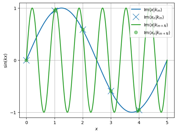
We stated that the peculiar index range considered above was equivalent to simply taking $m \in \{0, 1, \dots, N-1\}$, which demonstrates an important feature called aliasing. Although it seems like $k_{N-1}$ should have a high momentum

\[\begin{gather*} k_{N-1} = \frac{2\pi (N-1)}{L}, \end{gather*}\]

this is not seen because of the lattice. Specifically, $k_{n} \equiv k_{n\pm N}$:

\[\begin{gather*} \braket{x_{n}|k_{m\pm N}} = e^{\I k_{m \pm N} x_n} = e^{2\pi \I (m \pm N) n /N} = e^{2\pi \I mn /N \pm 2\pi \I n}\\ = e^{2\pi \I mn / N} = e^{\I k_{m}x_{n}} = \braket{x_{n}|k_{m}}. \end{gather*}\]

Viewed as a continuous function $\braket{x|k_{m+N}}$ has more rapid oscillations than $\braket{x|k_{m}}$, when evaluated on the lattice, we don’t see this.

N = 13
L = 10.0
x = np.linspace(-L, L, 500)[1:-1]
fig, ax = plt.subplots(figsize=(4, 3))
ax.plot(x/L, np.sin(np.pi * N * x / L) / np.sin(np.pi * x / L ) / N)
ax.set(xlabel="$x/L$", ylabel="$⟨x|x_0⟩$", title=f"{N=}");

_images/744c44c19fcb9f18fa64a6441f59cd3459ae6e2f98bd18d694b831e4205e4f4d.png

Basis Functions#

The exact basis functions considered here depend on the aliasing range. We can compute them:

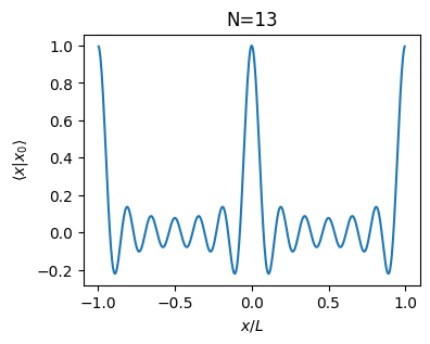
\[\begin{gather*} \braket{x|x_n} = \frac{1}{N}\sum_{l=m}^{m+N} \braket{x|k_l}\braket{k_l|x_n} = \frac{1}{N}\sum_{l=m}^{m+N} e^{\I k_l (x - x_n)} = \braket{x-x_n|x_0}. \end{gather*}\]

Thus, we see that all the basis functions are just shifted copies of one another. Now consider $\braket{x|x_0}$:

\[\begin{gather*} \braket{x|x_0} = \frac{1}{N}\sum_{l=m}^{m+N} e^{\I k_l x} = \frac{1}{N}\sum_{l=m}^{m+N} r^{l} = r^{m}\frac{r^{N} - 1}{r - 1}, \qquad r = e^{2\pi \I x/L},\\ \end{gather*}\]

To be explicit, consider $N$ odd such that $m=-(N-1)/2$ so that these functions are real. (The functions for even $N$ are similar, but contain a small imaginary component due to the asymmetric range of $k_l$.)

\[\begin{gather*} \braket{x|x_0} = \frac{1}{N}\frac{r^{N/2} - r^{-N/2}}{r^{1/2}-r^{-1/2}}, = \frac{1}{N}\frac{e^{\pi \I N x/L} - e^{-\pi \I N x/L}} {e^{\pi \I x/L} - e^{-\pi \I x / L}} = \frac{\sin(\pi N x/L)}{N\sin(\pi x/L)}. \end{gather*}\]

This is a periodic version of the $\sinc(\pi N x/L)$ function. Note that it has roots at all other abscissa $x_n$ except for $x=x_0$ where it is $1$.

Gibbs Phenomenon#

The Fourier basis of plane-waves is a complete countable basis for periodic functions and convergence pointwise as follows:

Theorem 5 (Dirichlet–Jordan test – Theorem 9.1.4 in [Hassani, 2013])

The Fourier series of a periodic function $f(x+L)=f(x)$ of bounded variation converges to

\[\begin{gather*} \frac{f(x + 0^+) + f(x - 0^+)}{2}. \end{gather*}\]

Here $f(x \pm 0^+) = \lim_{x\rightarrow x^{\pm}}f(x)$ is a shorthand for the directional limit.

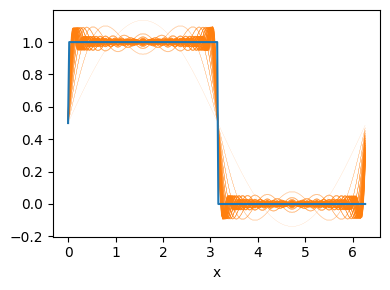
_images/7ee20e67236434b1d0dd6a9604d5a1808734446c40bf504303bc5d4b4d9403a7.png

This convergence is point-wise, but not necessarily uniform, as is demonstrated by the Gibbs phenomenon. As can be seen in the figure, the Fourier series always overshoots by about 18% at the discontinuity, no matter how many terms we include. Pointwise convergence is assured because the location of the overshoot moves closer and closer to the discontinuity.

Do It! Try to estimate the size of the overshoot.

Consider a discontinuity of strength $2\delta$ at $x=0$:

\[\begin{gather*} f(0^{\pm}) = \bar{f} \pm \delta. \end{gather*}\]

Integrating over this discontinuity over a region $x\in [-\epsilon, \epsilon]$, we have the following contribution to the Fourier coefficients:

\[\begin{gather*} \tilde{f}_{k} = C_k + \int_{-\epsilon}^{\epsilon}\d{x} e^{-\I k x}f(x)\\ \approx C_k + \frac{e^{-\I k \epsilon}f(0^+) - e^{\I k \epsilon}f(0^-)}{-\I k}\\ = C_k + \frac{2\bar{f}\sin(k \epsilon)}{k} - \frac{2\delta\cos(k\epsilon)}{\I k}. \end{gather*}\]

Assuming that the overshoot comes from this region, we can compute

\[\begin{gather*} \int\frac{\d{k}}{2\pi}\left( 2\bar{f}\frac{e^{\I k x}\sin(k\epsilon)}{k} - 2\delta\frac{e^{\I k x}\cos(k\epsilon)}{\I k}\right) = \end{gather*}\]

\[\begin{gather*} f(x) = \int\frac{\d{k}}{2\pi}e^{\I k x}\tilde{f}_k\\ \approx \int\frac{\d{k}}{2\pi}\left(e^{\I k x}C_k + 2\bar{f}\frac{e^{\I k x}\sin(k\epsilon)}{k} - 2\delta\frac{e^{\I k x}\cos(k\epsilon)}{\I k}\right). \end{gather*}\]

FFT#

We end by noting that the discrete Fourier transform and inverse Fourier transform are simply examples of matrix multiplication to change bases:

\[\begin{gather*} [\mat{F}]_{nm} = e^{-\I k_{m} x_{n}} = e^{-2\pi \I \frac{mn}{N}},\\ [\mat{F}^{-1}]_{nm} = \frac{1}{N}e^{\I k_{m} x_{n}} = \frac{1}{N}e^{2\pi \I \frac{mn}{N}}. \end{gather*}\]

We might thus expect that effecting one or the other transform would require $O(N^2)$ operations as is typical for matrix-vector multiplication. It turns out, however, that if $N$ can be factored into small primes – $N = 2^{n}$ is ideal – then one can use a clever divide-and-conquer algorithm call the fast Fourier transform which can compute this product in order $O(N\log N) operations. Efficient numerical implementations such as the FFTw keep the prefactor small, making this an excellent tool for numerical techniques if you can work with periodic bases.

Numerical Examples#

Sawtooth:

# Sawtooth Wave
L = 2*np.pi
N = 256
a = dx = L/N
x = np.arange(N) * dx
k = 2*np.pi * np.fft.fftfreq(N, dx)

# Here we use the mod function "%" to compute the square wave.
f = (x + np.pi) % (2*np.pi) - np.pi

# Use the FFT to compute the Fourier components
ft = np.fft.fft(f)

fig, axs = plt.subplots(1, 2, figsize=(10, 4))
ax = axs[0]
for n in range(2, 30):
    inds = np.where(abs(k) < 2*np.pi * (n+0.5)/L)[0]
    fn = (ft[inds, None] * np.exp(1j*k[inds, None]*x[None, :])).sum(axis=0).real/N
    ax.plot(x, fn, c='C1', lw=n/30)
ax.plot(x, f, 'C0-')
ax.set(xlabel="x")

ax = axs[1]
ax.loglog(abs(k), abs(ft), 'o-')
ax.set(xlabel=r"$|k|$", ylabel=r"$|\tilde{f}_{k}|$", aspect=1);
plt.tight_layout()

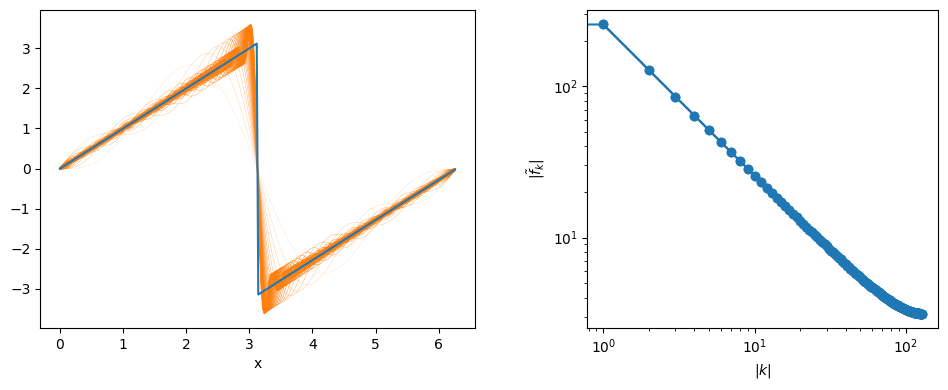
_images/4488472ad1d84dbb446a36f18ee5a6ad46e7731b5c7339704fecb2b0a577200f.png

Here we demonstrate the convergence to the sawtooth waveform on the left, and the $1/k$ dependence of the Fourier coefficients. Note, this is not exactly what is shown in Figure 19.1 of [Arfken et al., 2013] because we are working with the discrete Fourier transform – hence we also have a UV cutoff which the book does not include.

Square Wave:

# Square Wave
L = 2*np.pi
N = 256
a = dx = L/N
x = np.arange(N) * dx
k = 2*np.pi * np.fft.fftfreq(N, dx)

# Here we use the sign(x) function with a sine wave.

f = (1+np.sign(np.sin(x)))/2

# Use the FFT to compute the Fourier components
ft = np.fft.fft(f)

fig, axs = plt.subplots(1, 2, figsize=(10, 4))
ax = axs[0]
for n in range(2, 30):
    inds = np.where(abs(k) < 2*np.pi * (n+0.5)/L)[0]
    fn = (ft[inds, None] * np.exp(1j*k[inds, None]*x[None, :])).sum(axis=0).real/N
    ax.plot(x, fn, c='C1', lw=n/30)
ax.plot(x, f, 'C0-')
ax.set(xlabel="x")

ax = axs[1]
ax.loglog(abs(k), abs(ft), 'o-')
ax.set(xlabel=r"$|k|$", ylabel=r"$|\tilde{f}_{k}|$", aspect=1);
plt.tight_layout()

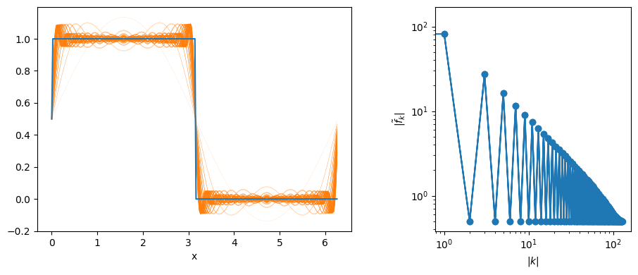
_images/a601d7eba2ba75d4b81d0e541ec164a4e8d93d0c19a079fbaca40b173478f4d5.png

Here we demonstrate the convergence to the square waveform on the left, and the $1/k$ dependence of the odd Fourier coefficients. Note, this is not exactly what is shown in Figure 19.7 of [Arfken et al., 2013] because we are working with the discrete Fourier transform – hence we also have a UV cutoff which the book does not include.

Convolution#

One of the most important properties of Fourier transforms is the convolution theorem. Let $\mathcal{F}(f)$ be the Fourier transform and $h=f*g$ be the convolution of functions $f$ and $g$:

\[\begin{gather*} \tilde{f} = \mathcal{F}(f), \qquad \tilde{f}_k \equiv \int_{-\infty}^{\infty}e^{-\I k x}f(x)\d{x}, \\ h = f*g, \qquad h(y) \equiv \int_{-\infty}^{\infty} f(x) g(y-x) \d{x}. \end{gather*}\]

Theorem 6 (Convolution)

The Fourier transform of a convolution $f*g$ is just the (elementwise) product of the Fourier transforms of the functions themselves:

\[\begin{gather*} \mathcal{F}(f*g) = \mathcal{F}(f)\mathcal{F}(g). \end{gather*}\]

Do It! Prove this

Hint: express $f$ and $g$ in terms of $\tilde{f}$ and $\tilde{g}$ using the inverse Fourier transform, then look for a Dirac delta function.

Application: Deconvolution#

As an application, consider looking at a galaxy with a telescope. If the optics in the telescope are linear, then $h(y)$ might represent the signal recorded on your CCD or film, while $f(x)$ is the actual picture of the galaxy. In this case, the function $g(x)$ represents the response of the telescope, which smears or blurs the image due to fact that the aperture is large, or the lens has imperfections.

Do It!

Show how to use the point spread function (PSF) to correct for the optics of the telescope by:

Measuring the PSF by looking at a point source.
Use the convolution theorem and Fourier transform of the PSF to recover the original signal $f(x)$ from the measured signal $h(y)$. Assume that both $f(x)$ and $h(y)$ go to zero far away from the object.
Check that this works numerically using numpy.fft.fft() and numpy.fft.ifft(). Note: you will have to make your functions periodic to use these. You can do this by padding them with zeros on both ends. How many zeros do you need to ensure that you don’t contaminate your results with aliasing artifacts?.

Application: Multiplication#

Another application is to multiply large numbers (integers). How many operations would it take to multiply two numbers with $N$ digits each using high-school techniques? (Answer: $O(N^2)$ operations.) Convince yourself that multiplication is really just convolution, hence one can use the FFT to perform the operation in $O(N\log N)$ time.

Application: Greens Functions#

Use Fourier techniques to solve the driven damped harmonic oscillator:

\[\begin{gather*} \ddot{q} + 2\beta \dot{q} + \omega_0^2 q = f(t) = \frac{F(t)}{m} \end{gather*}\]

where $f(t<0) = 0$ subject to the initial conditions $q(t<0) = 0$ and$ \dot{q}(t<0) = 0$.

Applications: PDEs#

Laplace Transform#

The Laplace transform of a function $f(t)$ is very closely related to the Fourier transform:

\[\begin{gather*} L(s) = \mathcal{L}\{f\}(s) = \int_0^{\infty}f(t) e^{-st}\d{t}. \end{gather*}\]

To see how this relates to the Fourier transform, and find the inverse transform, consider trying to transform a function like $f(t) = c$ or $f(t) = t^2$ where the Fourier transform does not converge. We might tame such integrals by introducing a weight $e^{-st}$ that decays as $x\rightarrow\infty$ and multiplying by the Heaviside step function:

\[\begin{gather*} H(x) = \begin{cases} 0 & x < 0\\ 1 & 0 < x. \end{cases} \end{gather*}\]

This might also be well motivated if the signal $f(t)$ is naturally zero for negative $t$ – such as a causal Green’s function. The Fourier transform of the modified signal becomes

\[\begin{gather*} F(\omega) = \mathcal{F}\{H(t)e^{-ct}f(t)\} = \int_{-\infty}^{\infty} H(t)f(t)e^{-ct} e^{-\I \omega t}\d{t} \end{gather*}\]

and the inverse transform is

\[\begin{gather*} H(t)f(t)e^{-ct} = \mathcal{F}^{-1}\{F(\omega)\}(t) = \int_{-\infty}^{\infty} F(\omega)e^{\I \omega t}\frac{\d{\omega}}{2\pi}. \end{gather*}\]

The Laplace transform comes from introducing the variable $s = c + \I \omega$:

\[\begin{gather*} L(s) = F(\omega) = \int_0^{\infty} f(t)e^{-st}\d{t}. \end{gather*}\]

The inverse Laplace transform is thus

\[\begin{gather*} f(t)H(t) = \int_{-\infty}^{\infty} F(\omega)e^{(\I \omega+c) t}\d{t}. = \int_{-\infty}^{\infty} F(\omega)e^{(\I \omega+c) t}\frac{\d{\omega}}{2\pi} = \int_{c-\I\infty}^{c+\I\infty} F(\omega)e^{s t}\frac{\d{s}}{2\pi \I}. \end{gather*}\]

I.e., this is a contour integral along a vertical line going through $\Re(s) = c$. The constant $c$ should be chosen so that it is greater than the real part of all singularities of $L(s)$ and $L(s)$ is bounded on the line. If $f(t<0) = 0$, then we can drop the factor of $H(t)$, giving the usual formula for the inverse Laplace transform.

Note that for real causal functions $f(t<0) = 0$, $F^*(\omega) = - F(\omega)$:

\[\begin{gather*} F^*(\omega) = \int_{-\infty}^{\infty} H(t)f(t)e^{-ct} e^{\I \omega t}\d{t} = -\int_{\infty}^{-\infty} H(t)f(t)e^{-ct} e^{\I \omega t}\d{t}\\ = \int_{-\infty}^{\infty} H(t)f(t)e^{-ct} e^{-\I \omega t}\d{t} = F(\omega). \end{gather*}\]