Bayesian Analysis and Bayes Factors

Bayesian Analysis and Bayes Factors#

Here we present some simple models to demonstrate and test Bayesian analysis. I am following some of the notations and discussions in [Turkman et al., 2019] as well as discussions in [Loredo, 1992] and [von Toussaint, 2011]. For a recent discussion, see also [Llorente et al., 2022].

Formulation#

Some notes: 1) As a physicist, I include the possibility of discrete parameters with finite probability by allowing the PDF to contain Dirac delta functions. 2) Often one will include additional conditional dependencies \(I\) in both the prior \(h(θ|I)\) and posterior \(h(θ|x,I)\) – after all, the choice of prior depends on something (e.g. previous measurements). We suppress this to simplify notation, but it should be kept in mind. 3) The marginal likelihood is also known as Bayesian evidence, model evidence, or sometimes simply evidence. 3) You will often see the likelihood function expressed as \(L(θ|x)\) (or \(\mathcal{L}(θ|x)\)) which I think comes from the idea of maximum likelihood estimation (MLE) in statistics where one maximizes over the parameters \(θ\) for fixed data \(x\). Note that \(L(θ|x)\) is not a PDF over \(θ\), but \(f(x|θ) = L(θ|x)\) is a PDF over \(x\). I thus, use the latter notation.

The basic idea is to express a model in terms of parameters \(θ\) drawn from some parameter space \(Θ\). Knowledge about the parameter values is expressed through various probability density functions (PDFs): specifically, prior knowledge \(h(θ)\), and posterior knowledge \(h(θ|x)\) incorporating some observations \(x\). Bayes’s theorem tells us how to use observations \(x\) to update the state of knowledge, obtaining the posterior distribution \(h(θ|x)\):

\[\begin{gather*} h(θ | x) = \frac{f(x|θ)h(θ)}{h(x)} \propto f(x|θ)h(θ), \qquad h(x) = \int f(x|θ)h(θ)\d{θ}, \end{gather*}\]

The model must also express the likelihood function \(f(x|θ)\), which is the probability of obtaining the observations \(x\) if the model parameters are \(θ\). In this sense, the observations \(x\) are a random variable \(X(θ)\) with an associated PDF \(f(x|θ)\).

The denominator \(h(x)\) is sometimes called the marginal likelihood. It is usually simply computed as a normalization factor to ensure that the posterior is a normalized probability distribution, and is omitted from discussions.

Warmup 1: The Proverbial Coin#

Consider flipping a coin, the outcomes of which are heads (\(x=1\)) with probability \(θ\), and tails (\(x=0\)) with probability \(1-θ\). What can you learn about \(θ\) by flipping the coin? Suppose you get \(N\) heads in a row. What is the 90% CI for \(θ\)?

The Bayesian approach first requires we specify a prior. Here we might assume we know nothing about \(θ\), and so take \(h(θ) \sim U(0, 1)\) to be uniform. The likelihood is straight-forward: assuming that the flips are independent, the likelihood of heads is simply \(θ\), so the likelihood of \(N\) heads in a row is \(f(x|θ) = θ^{N}\). Applying Bayes’ theorem, we have

\[\begin{gather*} h(θ|x) \propto f(x|θ)h(θ) = θ^{N}. \end{gather*}\]

Normalizing, we have

\[\begin{gather*} h(x) = \int_0^1 θ^{N}\d{θ} = \left.\frac{θ^{N+1}}{N+1}\right|_{0}^{1} = \frac{1}{N+1},\qquad h(θ|x) = (N+1)θ^{N}. \end{gather*}\]

ths = np.linspace(0, 1)
fig, ax = plt.subplots()
for N in range(5):
    ax.plot(ths, (N+1)*ths**N, label=f"{N=}")
ax.legend()
ax.set(xlabel="$θ$", ylabel="$h(θ|x)$", 
       title="Bayesian posterior after observing $N$ heads in a row.");

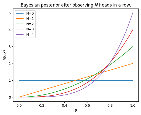
../_images/b7e203325122dbceda7f294311bd0c0227affdeb7951242e80f6371ebd3093a7.png

Generalizing, if out of \(N\) flips, one finds \(n\) heads, the posterior (with uniform prior) is the binomial distribution

\[\begin{gather*} h(θ|x) = \binom{N}{n} θ^n (1-θ)^{N-n}. \end{gather*}\]

The likelihood simply accumulates factors of \(θ\) and \((1-θ)\), independent of the order in which the data is taken.

To think about and discuss.

How does this treatment deal with the difference between the following observations:

Out of four flips, obtaining 2 heads and 2 tails. (There are \(\binom{4}{2} = 6\) ways to do this.)
Out of four flips, obtaining exactly the sequence HHTT. (There is exactly one way for this to occur.)

Warmup 2: Recognizable Subclasses#

[Jaynes and Kempthorne, 1976] has an interesting example that he presented at a convention of reliability and quality control statisticians working in the computer and aerospace industries:

at this point the meeting was thrown into an uproar, about a dozen people trying to shout me down at once. They told me, “This is complete nonsense. A method as firmly established and thoroughly worked over as confidence intervals couldn’t possibly do such a thing. You are maligning a very great man; Neyman would never have advocated a method that breaks down on such a simple problem. If you can’t do your arithmetic right, you have no business running around giving talks like this”… In the end they had to concede that my result was correct after all.

To make a long story short, my talk was extended to four hours (all afternoon), and their reaction finally changed to: “My God- why didn’t somebody tell me about these things before? My professors and textbooks never said anything about this. Now I have to go back home and recheck everything I’ve done for years”.

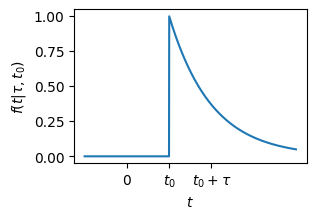
../_images/d1ce9cac07e496d512af03dc34c3708ecb1761177fa264c42ba69c6b673b5264.png

Jaynes’s example consists of a model with a PDF of

\[\begin{gather*} f(t|\tau, t_0) = p(t) = \frac{\Theta(t-t_0)}{\tau}e^{-(t-t_0)/\tau}. \end{gather*}\]

Physical interpretations include: random failure of a device after it runs out of a chemical inhibitor at time \(t_0\) [Jaynes and Kempthorne, 1976], or the observation of some astrophysical event whose first photons arrive at earth at time \(t_0\) [Loredo, 1992]. Prior to the event \(t < t_0\) there will be no detection, and after, there will be an exponentially decaying likelihood of detection.

Do it!

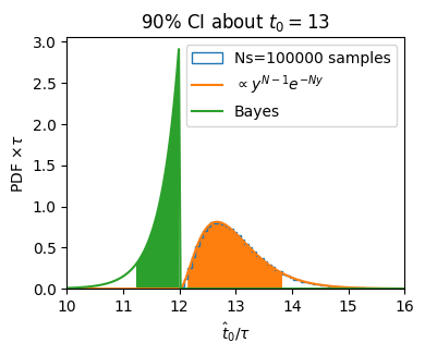
Assume that the decay constant \(\tau\) is known, and express all times in units of this (i.e. set \(\tau = 1\)). Determine a 90% CI for \(t_0\) given that the detector detects 3 photons at times \(t_i/\tau \in \{12, 14, 16\}\).

Although it is straightforward to simulate, this problem permits some analytic analysis. The population mean for the distribution is \( \braket{t} = t_0 + \tau\), thus, the shifted mean \(\hat{t}_0 = \braket{t - \tau}\) provides an unbiased estimator of \(t_0\):

\[\begin{gather*} \braket{t} = \int t p(t)\d{t} = t_0 + \tau, \qquad \hat{t}_0(\vect{t}) = \frac{1}{N}\sum_{i=1}^{N}(t_i - \tau). \end{gather*}\]

One can compute the distribution of the estimator if many samples of \(N\) detections are drawn from \(p(t)\), obtaining

\[\begin{gather*} p(\hat{t}_0|t_0) = \frac{1}{\tau}\frac{N^N}{\Gamma(N) }\Theta(y)y^{N-1}e^{-Ny}, \qquad y = \frac{\hat{t}_0 - t_0}{\tau} + 1 \end{gather*}\]

For the case in the problem of \(N=3\) one can also compute the CDF:

\[\begin{gather*} F(\hat{t}_0|t_0) = \int_{-\infty}^{\hat{t}_0}p(\hat{t}_0|t_0)\d{\hat{t}_0} = 1 - e^{-3y}\left(1 + 3y + \tfrac{9}{2}y^2\right). \end{gather*}\]

Since this is uni-modal, the 90% highest probability density CI is defined by values \(\hat{t}_{\pm}\) such that \(F_{N=3}(\hat{t}_+|t_0) - F_{N=3}(\hat{t}_-|t_0) = 0.9\) and \(p(\hat{t}_+|t_0) = p(\hat{t}_-|t_0)\). In terms of \(y_{\pm}\), this gives

\[\begin{gather*} y_-^2e^{-3y_-} = y_+^2e^{-3y_+}, \qquad - e^{-3y_{+}}(1 + 3y_{+}) + e^{-3y_{-}}(1 + 3y_{-}) = 0.9, \end{gather*}\]

which can be solved to find \(y \in [0.15, 1.83]\), or

\[\begin{gather*} t_0 \in [\braket{\hat{t}_0} + (0.15 - 1)\tau, \braket{\hat{t}_0} + (1.83 - 1)\tau]. \end{gather*}\]

For our example \(t_i/\tau \in \{12, 14, 16\}\), we have \(\braket{\hat{t}_0} = 13\tau\), and so our 90% CI is

\[\begin{gather*} \frac{t_0}{\tau} \in [12.15, 13.83]. \end{gather*}\]

As Jaynes and Loredo point out, this makes no sense since we know that \(t_0/\tau \leq 12\): The entire 90% CI lies in an impossible region!

The Bayesian approach is straightforward. In units with \(\tau = 1\), the likelihood is

\[\begin{gather*} f(\vect{t}|t_0) \propto \prod_{i=1}^{N}p(t_i|\tau, t_0) = Θ(12-t_0)e^{3(t_0-14)}. \end{gather*}\]

Given a uniform prior \(h(t_0) \propto 1\), we find the Bayesian posterior given the data to be (in units where \(\tau=1\)):

\[\begin{gather*} h(t_0|\vect{t}) = Θ(12-t_0)3e^{6}e^{3(t_0-14)}. \end{gather*}\]

This properly excludes \(t_0 > 12\). Computing the 90% highest probability density CI, we find:

\[\begin{gather*} \frac{t_0}{\tau} \in [11.23, 12]. \end{gather*}\]

Details.

The cumulative distribution is

\[\begin{gather*} C(t_0|\vect{t}) = \int_{-\infty}^{t_0}\d{t}\; h(t|\vect{t}) = \begin{cases} e^{3(t_0 - 12)} & t_0 < 12\,,\\ 1 & \text{otherwise}. \end{cases} \end{gather*}\]

The mode is at \(t_0 = t_+ = 12\) and the 90% confidence interval can be found by finding where \(C(t_{-}|\vect{t}) = 10\%\):

\[\begin{gather*} 0.1 = e^{3(t_0 - 12)} t_{-} = 12 + \frac{\ln 0.1}{3} = 11.96\dots. \end{gather*}\]

../_images/307e5f13a14acd4d7ce06713d86c42c28f2e79d13b0dc4e2e585d8e5b8c5c78a.png

The problem here is that the particular observation at hand is actually extremely unlikely, thus the typical statistical analysis – which is based on typical outcomes – gives wildly inaccurate results.

Simple Problem#

We start with a simple problem. Consider measuring a value \(θ\) where the measurement process introduces an error \(\eta\) with PDF \(f(\eta)\):

\[\begin{gather*} x = θ + \eta, \qquad \eta \sim f(\eta). \end{gather*}\]

Consider two models: one where \(θ \in [0, 1]\) is a real number, and another where \(θ\in \{0, 1/2, 1\}\) is discrete. Can we learn about which model is better by analyzing some data?

Let’s start with the standard approach, assuming a flat prior \(θ \sim U(0, 1)\):

\[\begin{align*} h(θ) &= \begin{cases} 1 & 0 \leq θ \leq 1\\ 0 & \text{otherwise}, \end{cases}, & h(θ) &= \frac{1}{3}\Bigl(\delta(a) + \delta(a-0.5) + \delta(a-1)\Bigr). \end{align*}\]

Given a value \(a\), the likelihood of measuring \(x\) is:

\[\begin{gather*} L(x|a) = f(x-a) \end{gather*}\]

from our model. Thus, our posterior after \(N\) independent measurements \(\vect{x}\) is

\[\begin{gather*} p_{\vect{x}}(a) \propto \underbrace{\prod_{n}p_{\eta}(x_n - a)}_{\mathcal{L}(\vect{x}|a)} p_0(a) \end{gather*}\]

Polynomial Fitting#

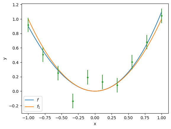
We will consider data sampled from three different functional models:

\[\begin{gather*} f_1(x) = ax^2\\ f_2(x) = ax^2 + bx^3\\ f_3(x) = ax^2 + bx^3 + cx^4\\ g(x) = 1 - A\cos(Bx + C) \end{gather*}\]

We will generate data from model \(f_2\), and would like to used Bayesian techniques to compare the models to develop an intuition about when data can exclude models \(f_1\) and \(g\), etc.

A First Approach#

Let’s start by generating some data. We will take the following values:

\[\begin{gather*} a = 1, \qquad b = 0.1, \qquad c = 0. \end{gather*}\]

%matplotlib inline
import numpy as np, matplotlib.pyplot as plt
#plt.rcParams['figure.figsize'] = (4, 3)

a, b, c = 1, 0.1, 0
dy = 0.1

def f(x, a=1, b=0.1, c=0):
    """Return f(x), the model function."""
    return a*x**2 + b*x**3 + c*x**4

def get_data(x, f, dy=0.1, seed=2):
    """Return some data with gaussian errors."""
    # Use a seed so results are reproducible
    rng = np.random.default_rng(seed=seed)
    y = f(x) + rng.normal(scale=dy, size=x.shape)
    return y

x = np.linspace(-1, 1, 10)
x_ = np.linspace(-1, 1, 100)

y = get_data(x, f, dy=dy)
fig, ax = plt.subplots()

ax.plot(x_, f(x_), label="$f$")
ax.plot(x_, f(x_, a=a, b=0, c=0), label="$f_1$")
ax.errorbar(x, y, yerr=dy, fmt='.');
ax.legend()
ax.set(xlabel='x', ylabel='y');

../_images/27685f782aa4002c490f0e959c04c718d854c577843c5b243c649fe042c30a99.png

Since everything is linear and Gaussian, the standard least-squares regression should work. See scipy.optimize.curve_fit.

from scipy.optimize import curve_fit
import scipy
p_opt, p_cov = curve_fit(f, x, y, sigma=dy, 
                         absolute_sigma=True)
print(p_opt), print(np.sqrt(np.diag(p_cov)))
chi_r = np.sqrt(sum(((f(x, *p_opt) - y)/dy)**2) / (len(y) - len(p_opt)))
chi_r

[0.91435803 0.09666077 0.07401629]
[0.22123447 0.06319118 0.25119305]

np.float64(1.3003693229853386)

Odds and Ends#

Credible Intervals (Confidence Intervals)#

A proper characterization of a Bayesian analysis is by describing the posterior distribution, but one often desires a simpler characterization. For a single parameter \(θ\) with posterior \(h(θ | x)\), one might report a “95% credible interval \([\underline{θ}, \overline{θ}]\)” meaning

\[\begin{gather*} \int_{\underline{θ}}^{\overline{θ}}h(θ | x)\d{θ} = 0.95 = 1-\alpha. \end{gather*}\]

However, the choice of \(\underline{θ}\) and \(\overline{θ}\) satisfying this is not unique. One possibility is a symmetric interval

\[\begin{gather*} \int_{-\infty}^{\underline{θ}}h(θ | x)\d{θ} = \int_{\overline{θ}}^{\infty}h(θ | x)\d{θ} = \frac{1-0.95}{2} = \frac{\alpha}{2}. \end{gather*}\]

This does not generalize to higher dimensions.

The preferred way is to define the highest posterior density (HPD) credible set \(A = \{θ \mid h(θ | x) \geq k\}\) where \(k\) is the largest real number such that \(P(A) \geq 0.95 = 1-\alpha\). This generalizes, but is sensitive to the choice of parameter \(θ\). Choosing a different parameterization will usually change the HPD credible set.

Bayes Factor#

Bayes theorem is

\[\begin{gather*} h(θ | x) \propto L(x | θ) h(θ). \end{gather*}\]

For a Bayesian, two competing “models” or hypotheses might consist of disjoint parameter regimes \(Θ_0 \cap Θ_1 = \emptyset\) and \(Θ_0 \cup Θ_1\) is the full parameter space. The probability of these competing hypotheses is

\[\begin{gather*} P(Θ_{i}) = \int_{Θ_{i}} h(θ)\d{θ}, \qquad P(Θ_{i}|x) = \int_{Θ_{i}} h(θ|x)\d{θ}. \end{gather*}\]

The Bayes factor is

\[\begin{gather*} B(x) = \frac{P(Θ_0|x) / P(Θ_0)} {P(Θ_1|x) / P(Θ_1)}. \end{gather*}\]

The larger \(B(x)\), the more the data \(x\) supports hypothesis \(Θ_0\). Part of the goal of this exercise is to develop some intuition about what this means.

Questions

Q: What happens if the hypotheses or models overlap? How does the polynomial model-selection fit into this formalism? A: Apparently one should make sure that all models are part of the same space to use Bayes factors.

Problem 1.4

Given a coin which lands with probability \(θ\) as heads. The problem asks us to test three hypotheses \(Θ_<\), \(Θ_=\), and \(Θ_>\), that \(θ < 0.5\), \(θ = 0.5\), and \(θ > 0.5\) respectively (slightly changed notation). The problem asks us to assume prior probabilities to the hypotheses \(P(Θ_<) = P(Θ_>) = 0.25\) and \(P(Θ_=) = 0.5\) with corresponding uniform priors \(h(θ \mid Θ_<) = U(0, 0.5)\), \(h(θ \mid H_{>}) = U(0.5, 1)\).

After flipping the coin once and finding heads \(x_0 = h\), we are asked to compute the Bayes factors for the various hypotheses.

First some notations: From the discussion above, we can express the hypotheses as sets \(Θ_{<} = [0, 0.5)\), \(Θ_{>} = (0.5, 1]\), and \(Θ_{=} = \{0.5\}\) with prior

\[\begin{gather*} h(θ) = \frac{1}{2} + \frac{\delta(θ - 0.5)}{2}. \end{gather*}\]

Note that the prior probabilities are just the corresponding “areas”:

\[\begin{gather*} 1 = \int_{0}^{1}h(θ)\d{θ} = \underbrace{\int_{0}^{0.5-0^+}h(θ)\d{θ}}_{P(Θ_<)=1/4} + \underbrace{\int_{0.5-0^+}^{0.5+0^+}h(θ)\d{θ}}_{P(Θ_=)=1/2} + \underbrace{\int_{0.5+0^+}^{1}h(θ)\d{θ}}_{P(Θ_>)=1/4}\,. \end{gather*}\]

The likelihood of getting heads is just \(θ\)

\[\begin{gather*} L(h | θ) = θ\,. \end{gather*}\]

Thus, the normalized posterior distribution is

\[\begin{gather*} h(θ | h) = θ\Bigl(1 + \delta(θ - 0.5)\Bigr) \propto L(h | θ)h(θ). \end{gather*}\]

For further flips, the posterior after \(N\) flips with \(n\) heads is

\[\begin{gather*} h(θ | \vect{x}) \propto θ^{n}(1-θ)^{N-n}\Bigl(1 + \delta(θ - 0.5)\Bigr). \end{gather*}\]

We can now compute the various probabilities of the competing hypotheses after the flip:

\[\begin{gather*} 1 = \int_{0}^{1}h(θ)\d{θ} = \overbrace{\int_{Θ_<} h(θ)\d{θ}}^{P(Θ_{<})=1/4} + \overbrace{\int_{Θ_=} h(θ)\d{θ}}^{P(Θ_{=})=1/2} + \overbrace{\int_{Θ_>} h(θ)\d{θ}}^{P(Θ_{>})=1/4}\,,\\ 1 = \int_{0}^{1}h(θ | h)\d{θ} = \underbrace{\int_{Θ_<} h(θ|h)\d{θ}}_{P(Θ_{<}|h)=1/8} + \underbrace{\int_{Θ_=} h(θ|h)\d{θ}}_{P(Θ_{=}|h)=1/2} + \underbrace{\int_{Θ_>} h(θ|h)\d{θ}}_{P(Θ_{>}|h)=3/8}\,. \end{gather*}\]

The relative Bayes factors are thus

\[\begin{gather*} B_{< \text{ vs } =} = \frac{(1/8) / (1/2)}{(1/4) / (1/2)} = \frac{1}{2} = 0.5,\\ B_{> \text{ vs } =} = \frac{(3/8) / (1/2)}{(1/4) / (1/2)} = \frac{3}{2} = 1.5,\\ B_{> \text{ vs } <} = \frac{(3/8) / (1/8)}{(1/4) / (1/4)} = 3. \end{gather*}\]