Show code cell content

Hide code cell content

%matplotlib inline
import numpy as np, matplotlib.pyplot as plt

plt.rcParams['figure.figsize'] = (4, 3)

Drums

Consider a thin 2D drum-head streched taught over a frame outlining some specified region of the \(x\)-\(y\) plane. Small-amplitude oscillations of the drum can be described by their height \(f(x,y,t)\) and will satisfy the 2D wave equation:

\[\begin{gather*} \pdiff[2]{}{t}f(x,y,t) = c^2\nabla^2 f(x,y,t) \end{gather*}\]

where \(c\) is the speed of sound in the material which will depend on the tension and mass density of the drumhead (assumed to be uniform). The solutions must satisfy the boundary condition \(f(x,y,t) = 0\) wherever the point \((x,y)\) lies on (or outside) of this region. (These are called Dirichlet boundary conditions.).

We start with a brute-force solution that, while computationally expensive, will allow us to solve for the modes of an arbitrary region. To do this, we first discretize the problem by tabulating the function at a set of equally spaced points \((x_m, y_n)\) in the plane with spacing \(x_{m+1} - x_{m} = \delta x\) and \(y_{n+1} - y_n = \delta y\).

The strategy will be to formulate a matrix representation of the laplacian \(\nabla^2\) and then look for eigenfunctions \(\nabla^2 f_n = -\frac{\omega^2_n}{c^2} f_n\). From these eigenfunctions we can form the time-dependent solutions:

\[\begin{gather*} f(x,y,t) = \Re\left(\sum_{n} a_n e^{\I\omega_n t} f_n(x,y)\right) \end{gather*}\]

where \(a_n\) are arbitrary complex coefficients.

This notebook demonstrates a very general method (but with low accuracy) for finding the eigenmodes. Along the way, we will explore finite-difference approximations to the second derivative (Laplacian) with a discussion about their error scaling.

TL:DR

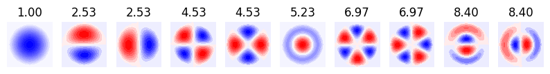
Here is a quick and dirty solution for a circular drum head whose analytic solution is

\[\begin{gather*} \psi_{mn}(r, \phi, t) = \Re \Bigl( J_{\abs{m}}(k_nr) e^{\I m\phi} e^{\I\omega t} \Bigr), \qquad \omega^2 = c^2k_n^2, \qquad J_{\abs{m}}(k_nR) = 0. \end{gather*}\]

Details will be presented below

%matplotlib inline
import numpy as np, matplotlib.pyplot as plt
from scipy import special

L = 2.2  # Size of box
R = 1.0  # Radius of drum head
N = 32  # Number of points
h = L / N  # Lattice spacing

# The abscissa are adjusted so that zero is in the center
x = y = np.arange(N) * h - L / 2.0 + h / 2.0
X = x[:, None]
Y = y[None, :]

# Here is the matrix D2 expressing Dirichlet boundary conditions
# Note that np.eye() returns an "identity" matrix with ones on
# the k'th diagonal
d2 = (np.eye(N, k=1) + np.eye(N, k=-1) - 2 * np.eye(N)) / h**2

# Here we form the tensor product using Einstein notation
D2x = np.einsum('ab,ij->aibj', d2, np.eye(N))
D2y = np.einsum('ab,ij->iajb', d2, np.eye(N))
D2 = (D2x + D2y).reshape((N**2, ) * 2)

# Get the indices into the 1D ravelled array where the membrane can fluctuate:
inds = np.where((X**2 + Y**2 < R**2).ravel())[0]

# Now restrict the Laplacian to these indices:
D2_ = D2[inds, :][:, inds]

# Make sure it is Hermitian
assert np.allclose(D2_, D2_.T)

# Find modes by diagonalizing the negative of the matrix
# so that the modes are sorted by energy
Es, Vs = np.linalg.eigh(-D2_)

# Plot several modes
modes = 10
#fig, axs = plt.subplots(2, modes, figsize=(modes, 4))  # Make figure wide enough.
fig, axs = plt.subplots(1, modes, figsize=(modes, 4))  # Make figure wide enough.
for n in range(modes):
    ax = axs[n]
    f = np.zeros((N, N))     # Full grid of zeros
    f.flat[inds] = Vs[:, n]  # Insert active points into f
    f_ = abs(f).max()        # Normalize colors so white is zero
    
    ax.contourf(
        x,
        y,           # Filled contour plot.
        f.T,         # Transpose because this follows MATLAB's conventions
        15,          # Number of contours
        cmap='bwr',  # Divergent colormap to show both + and - clearly
        vmin=-f_,    # These need to be set so that 0 is in the middle of the map 
        vmax=f_)     #   and appears white in the plots
    ax.set(aspect=1, # Make circles circular
           title=f"{Es[n]/Es[0]:.2f}")  # Energy as title
    ax.set_axis_off()  # Turn off ticks, numbers, etc.

Laplacian in 1D

The challenge is to find a matrix representation of the laplacian. We start with the form in 1D which is just the second derivative operator. Expending in terms of the lattice spacing \(h\) we have the following Taylor series:

\[\begin{gather*} f(x \pm h) = f(x) \pm hf'(x) + \frac{h^2}{2}f''(x) \pm \frac{h^3}{3!}f'''(x) + \cdots. \end{gather*}\]

This allows us to define the following finite difference approximation for the second derivative:

\[\begin{gather*} \mat{D}_2\cdot f = \frac{f(x+h) + f(x-h) - 2f(x)}{h^2} = f''(x) + \frac{h^2}{12} f''''(x) + \cdots. \end{gather*}\]

This is a second order finite-difference approximation and the error scales as \(h^2\) as shown. As a matrix, this operator looks like:

\[\begin{gather*} \mat{D}_2 = \frac{1}{h^2}\begin{pmatrix} \ddots & \ddots\\ \ddots & -2 & 1\\ & 1 & -2 & 1\\ & & 1 & -2 & 1\\ & & & 1 & -2 & \ddots \\ & & & & \ddots & \ddots \end{pmatrix} \end{gather*}\]

If one needs higher accuracy, then one can include more terms. For example:

\[\begin{gather*} f''(x) = \frac{-30f(x)+16[f(x+h) + f(x-h)] - f(x+2h)- f(x-2h)}{12h^2} + \order(h^4) \end{gather*}\]

\[\begin{gather*} \mat{D}_2 = \frac{1}{12h^2}\begin{pmatrix} \ddots & \ddots & \ddots\\ \ddots & -30 & 16 & -1\\ \ddots & 16 & -30 & 16 & -1\\ & -1 & 16 & -30 & 16 & \ddots\\ & & -1 & 16 & -30 & \ddots\\ & & & \ddots & \ddots & \ddots \end{pmatrix} \end{gather*}\]

Boundary Conditions

To finish defining the matrix \(\mat{D}_2\) we need to specify what happens at the boundaries. There are four common sets of boundary conditions:

• Periodic: \(f(0) = f(L)\).

• Dirichlet: \(f(0) = 0\).

• Neumann: \(f'(0) = 0\).

• Free: \(f''(0) = 0\).

These boundary conditions can be applied at either end of the interval \(x=0\) or \(x=L\) and can be mixed. Note that a fifth type – clamped – where \(f(0) = f_0 \neq 0\) is held fixed should be implemented by first finding a particular solution to \(\nabla^2 f_0 = 0\) which satisfies the boundary conditions, and then adding solutions that satisfy the Dirichlet condition. Thus, the excitation pattern is the same as for Dirichlet conditions. For 1D, such a particular solution would be \(f_0(x) = f_N\frac{x-x_{-1}}{x_{N} - x_{-1}} + f_{-1}\frac{x_{N} - x}{x_{N} - x_{-1}}\). In higher dimensions the problem is not so trivial and one must first find a particular solution the \(\nabla^2 f_0 = 0\) to add that satisfies the boundary conditions. Note that this does not affect the pattern of nodes, however, so we do not consider this case further.

To implement these numerically it is often easiest to think of the matrix \(\mat{D}_2\) acting on an augmented set of points just outside of the interval of solution (colored in red below). Recall that in python we index our points from \(n=0\) to \(n=N-1\), so this means considering the points \(f_{-1} = f(x_{-1})\) and \(f_{N} = f(x_{N})\):

\[\begin{gather*} \begin{pmatrix} \red{f''_{-1}}\\ f''_0\\ f''_1\\ \vdots\\ f''_{N-1}\\ \red{f''_{N}} \end{pmatrix} \approx \frac{1}{h^2} \begin{pmatrix} \red{-2} & \red{1}\\ \red{1} & -2 & 1\\ & 1 & \ddots & \ddots\\ & & \ddots & \ddots & 1 \\ & & & 1 & -2 & \red{1}\\ & & & & \red{1} & \red{-2} \end{pmatrix} \cdot \begin{pmatrix} \red{f_{-1}}\\ f_0\\ f_1\\ \vdots\\ f_{N-1}\\ \red{f_{N}} \end{pmatrix} \end{gather*}\]

Now one can simply set the appropriate values for \(f_{-1}\) and \(f_{N}\) to obtain the required matrix \(\mat{D}_2\):

• Periodic: \(f_{-1} = f_{N-1}\) and \(f_{N} = f_{0}\).

  \[\begin{gather*} \begin{pmatrix} f''_0\\ f''_1\\ \vdots\\ f''_{N-1} \end{pmatrix} \approx \frac{1}{h^2} \begin{pmatrix} \red{1} & -2 & 1\\ & 1 & \ddots & \ddots\\ & & \ddots & -2 & 1 \\ & & & 1 & -2 & \red{1}\\ \end{pmatrix} \cdot \begin{pmatrix} \red{f_{N-1}}\\ f_0\\ f_1\\ \vdots\\ f_{N-1}\\ \red{f_{0}} \end{pmatrix} \quad \implies \quad \mat{D}_2 = \frac{1}{h^2}\begin{pmatrix} -2 & 1 & & \green{1}\\ 1 & \ddots & \ddots\\ & \ddots & \ddots & 1\\ \green{1} & & 1 & -2 \end{pmatrix} \end{gather*}\]

• Dirichlet: \(f_{-1} = f_{N} = 0\).

  \[\begin{gather*} \begin{pmatrix} f''_0\\ f''_1\\ \vdots\\ f''_{N-1} \end{pmatrix} \approx \frac{1}{h^2} \begin{pmatrix} \red{1} & -2 & 1\\ & 1 & \ddots & \ddots\\ & & \ddots & -2 & 1 \\ & & & 1 & -2 & \red{1}\\ \end{pmatrix} \cdot \begin{pmatrix} \red{0}\\ f_0\\ f_1\\ \vdots\\ f_{N-1}\\ \red{0} \end{pmatrix} \quad \implies \quad \mat{D}_2 = \frac{1}{h^2}\begin{pmatrix} -2 & 1\\ 1 & \ddots & \ddots\\ & \ddots & \ddots & 1\\ & & 1 & -2 \end{pmatrix} \end{gather*}\]

• Neumann: \(f'_{-1} = f'_{N} = 0\). This case is a little subtle. Naively one might think that setting \(f_{-1} = f_0\) and \(f_{N-1} = f_{N}\) would be enough to ensure the condition \(f'=0\) at the boundaries:

  \[\begin{gather*} \begin{pmatrix} f''_0\\ f''_1\\ \vdots\\ f''_{N-1} \end{pmatrix} \approx \frac{1}{h^2} \begin{pmatrix} \red{1} & -2 & 1\\ & 1 & \ddots & \ddots\\ & & \ddots & -2 & 1 \\ & & & 1 & -2 & \red{1}\\ \end{pmatrix} \cdot \begin{pmatrix} \red{f_0}\\ f_0\\ f_1\\ \vdots\\ f_{N-1}\\ \red{f_{N-1}} \end{pmatrix} \quad \implies \quad \mat{D}_2 = \frac{1}{h^2}\begin{pmatrix} \green{-1} & 1\\ 1 & \ddots & \ddots\\ & \ddots & \ddots & 1\\ & & 1 & \green{-1} \end{pmatrix}. \end{gather*}\]

  This approximation at the endpoints uses the formula \(f'_{-1} = (f_{0} - f_{-1})/h + \order(h)\) which is only acurrate to order \(\order(h)\). Unfortunately, this spoils the accuracy of the entire approach, making it only accurate to \(\order(h)\) rather than order \(\order(h^2)\). There are two solutions:

  1. The first approach is to note that the approximation \(f_{-1/2} = (f_{0} - f_{-1})/h + \order(h^2)\) is accurate to second order at the midpoint between \(x_{-1}\) and \(x_{0}\). Thus, we can use the same matrix derived above, but we must be careful to define our lattice so that the boundary conditions are applied at the midpoint between the last lattice point and then next one.

  2. The second approach is to use an order \(\order(h^2)\) approximation for the derivatives at the endpoints. The following works:

     \[\begin{gather*} f'_{-1} = \frac{4f_0 - 3f_{-1} - f_{1}}{2h} + \order(h^2). \end{gather*}\]

     Setting this to zero gives the condition \(f_{-1} = \frac{4f_0 - f_1}{3}\).

     \[\begin{gather*} \begin{pmatrix} f''_0\\ f''_1\\ \vdots\\ f''_{N-1} \end{pmatrix} \approx \frac{1}{h^2} \begin{pmatrix} \red{1} & -2 & 1\\ & 1 & \ddots & \ddots\\ & & \ddots & -2 & 1 \\ & & & 1 & -2 & \red{1}\\ \end{pmatrix} \cdot \begin{pmatrix} \red{(4f_0-f_1)/3}\\ f_0\\ f_1\\ \vdots\\ f_{N-1}\\ \red{(4f_{N-1}-f_{N-2})/3} \end{pmatrix} \quad \implies \quad \mat{D}_2 = \frac{1}{h^2}\begin{pmatrix} \green{-2/3} & \green{2/3}\\ 1 & \ddots & \ddots\\ & \ddots & \ddots & 1\\ & & \green{2/3} & \green{-2/3} \end{pmatrix}. \end{gather*}\]

     The disadvantage of this approach is that the resulting matrix is no-longer symmetric, which can make it more difficult to work with numerically.

%pylab inline --no-import-all
import os.path, sys
sys.path.append(os.path.expanduser('~/.local/lib/python3.5/site-packages/'))

%pylab is deprecated, use %matplotlib inline and import the required libraries.
Populating the interactive namespace from numpy and matplotlib

Periodic

For periodic boundary conditions \(f(x+L) = f(x)\), we have \(f_{N} = f_{0}\) which means that the points on either end of our abscissa correspond to the first or last abscissa points. This means that if we have \(N\) points in our basis, then the lattice spacing is \(h = L/N\) and the periodic box length is \(L\). One can cnoose different conventions about the location of the abscissa. In our case, we will center then in the middle of our box:

\[\begin{gather*} x_{n} = hn - \frac{L}{2} + \frac{h}{2}. \end{gather*}\]

If we omit the last term, then the abscissa will include the left endpoint of the box but not the right endpoint (which is a perfectly valid choice too.)

def get_periodic(N=64, L=2.2, order=2):
    """Return `(x, d2)` for a periodic box.

    Arguments
    ---------
    N : int
       Number of points
    L : float
       Length of the box

    Returns
    -------
    x : 1d-array
       The abscissa centered in the box.
    d2 : 2d-array
       The laplacian operator in this basis
    """
    h = L / N
    x = np.arange(N) * h - L / 2.0 + h / 2.0
    if order == 2:
        d2 = (-2 * np.eye(N) + np.eye(N, k=1) + np.eye(N, k=-1)) / h**2
        d2[0, -1] = d2[-1, 0] = 1. / h**2
    elif order == 4:
        d2 = -15 * np.eye(N) + 16 * np.eye(N, k=1) - np.eye(N, k=2)
        d2[0, -1] = 16
        d2[1, -1] = d2[0, -2] = -1
        d2 = (d2 + d2.T) / (12.0 * h**2)
    else:
        raise NotImplementedError
    return x, d2

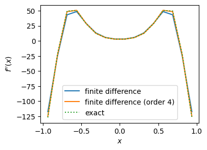
Testing

When implementing a numerical method, it is important to test your results. Here we use the following function to test our code. Note: for accuracy we must make sure that the function satisfies periodic boundary conditions implied by our choice of basis:

\[\begin{gather*} c = \cos\frac{2\pi x}{L}, \qquad s = \sin\frac{2\pi x}{L},\\ f_p(x) = e^{-ac/2}, \qquad f_p'(x) = \frac{a\pi}{L}s, \qquad f_p''(x) = \frac{a\pi^2}{L^2}(as^2 + 2c)f(x). \end{gather*}\]

def get_f(x, L, a=4.0, d=0):
    """Return the d'th derivative of the test function."""
    c = np.cos(2*np.pi*x/L)
    s = np.sin(2*np.pi*x/L)
    f = np.exp(-a*c/2.0)
    if d == 0:
        return f
    elif d == 1:
        return a*np.pi/L*s*f
    elif d == 2:
        return a*(np.pi/L)**2*(a*s**2 + 2*c)*f
    else:
        raise NotImplementedError

L = 2.0
N = 16
x, d2 = get_periodic(N=N, L=L)
x, d2_ = get_periodic(N=N, L=L, order=4)
f = get_f(x, L, d=0)
d2f = get_f(x, L, d=2)
fig, ax = plt.subplots()
ax.plot(x, d2.dot(f), '-', label='finite difference')
ax.plot(x, d2_.dot(f), '-', label='finite difference (order 4)')
ax.plot(x, d2f, ':', label='exact')
ax.legend(loc='best')
ax.set(xlabel='$x$', ylabel=r"$f''(x)$");

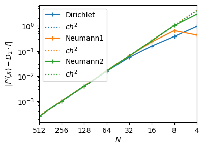
Now we check the scaling of the errors with the basis size. We expect from our results above that the errors should scale as \(h^2\)so if we plot this on a log-log plot, we should see:

\[\begin{gather*} \text{err} = c h^2, \qquad \log(\text{err}) = \log(c) + 2 \log(h) \end{gather*}\]

where the coefficient \(c\) depends on properties of the function.

For comparison, we provide a different implementation of the Laplacian that uses the fast Fourier transform (FFT). If you have a periodic function that is smooth (analytic) this it is almost always preferable to use Fourier (spectral) methods as will become clear shortly. Unfortunately, these methods do not work well with the irregular boundary conditions we use here for drums since the functions are non-analytic at the boundaries.

L = 2.0


def _d2(f):
    """Compute the Laplacian using Fourier techniques."""
    N = len(f)
    dx = L / N
    k = 2 * np.pi * np.fft.fftfreq(N, dx)
    return np.fft.ifft(-k**2 * np.fft.fft(f)).real


Ns = 2**np.arange(2, 10)
hs = L / Ns
errs = []
errs4 = []
errs_fourier = []
for N in Ns:
    x, d2 = get_periodic(N=N, L=L)
    x, d2_ = get_periodic(N=N, L=L, order=4)
    f = get_f(x, L, d=0)
    d2f = get_f(x, L, d=2)
    errs.append(abs(d2.dot(f) - d2f).max())
    errs4.append(abs(d2_.dot(f) - d2f).max())
    errs_fourier.append(abs(_d2(f) - d2f).max())

errs = np.array(errs)  # Make errs a numpy array so we can compute with it

# Estimate slope by fitting a polynomial to the two smallest points
slope, logc = np.polyfit(np.log10(hs[-2:]), np.log10(errs[-2:]), 1)
slope4, logc4 = np.polyfit(np.log10(hs[-2:]), np.log10(errs4[-2:]), 1)
fig, ax = plt.subplots()
ax.loglog(hs, errs, '-+b', label='error')
ax.loglog(hs, 10**logc * hs**2, ':b', label=r'$ch^2$')
ax.loglog(hs, errs4, '-+k', label='error (order 4)')
ax.loglog(hs, 10**logc4 * hs**4, ':k', label=r'$ch^4$')
ax.loglog(hs, errs_fourier, '--+g', label='error (Fourier)')
ax.set_xscale('log', base=2)
ax.legend(loc='lower left')
ax.set(xlabel='$N$',
       ylabel=r"$|f''(x) - D_2\cdot f|$",
       xlim=(hs.min(), hs.max()),
       xticks=hs,
       xticklabels=Ns);  # Show N instead of h on bottom axis

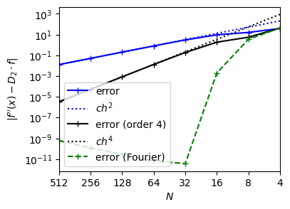
From this we notice two several general features:

• We see the method follows the \(h^2\) scaling as expected.

• However, we see that the accuracy is very poor: even \(N=512\) points, we only realize an answer accurate to two decimal places. To realize 6 places of accuracy, for example, would require \(N=2^{16} = 65536\) points. For our drum problem we need a matrix which has about \(N^2 = 2^{32}\) floating point numbers, or about \(32\)GB of storage.

• The higher order method performs better, almost reaching 6 places of accurcay at \(N=512\), but is still quite slow to converge.

• In comparison, the Fourier method has realized maximum precision (12 digits) by \(N=32\) points, at which point roundoff error dominates the calculations. Where possible, use Fourier techniques, but they only achieve such high precision if the functions are truely periodic and smooth (analytic). For this work, we will not be able to benefit from this since the drums are clampped at the boundaries, which introduces non-analytic behavior in \(f(x,y)\) in the form of a kink.

Dirichlet and Neumann

For the Neumann boundary conditions we must modify the lattice. The strategy that we take is to define indices \(n_l\) and \(n_r\) at which the boundary conditions apply. For Dirichlet and Neumann2, we have \(n_l = 0\) and \(n_r = N-1\). For Neumann1 we have \(n_l = -1/2\) and \(n_r = N-1/2\). Once these are fixed, we have:

\[\begin{gather*} h n_l + b = -\frac{L}{2}, \qquad h n_r + b = \frac{L}{2}, \\ h = \frac{L}{n_r-n_l}, \qquad b = -\frac{L}{2} - hn_l \end{gather*}\]

def get_fixed(N=64, L=2.2, type=('Dirichlet', 'Dirichlet')):
    """Return `(x, d2)` for a periodic box.

    Arguments
    ---------
    N : int
       Number of points
    L : float
       Length of the box
    type : (left, right)
       Specify the type of boundary condition on the left and right:
       'Dirichlet' or 'Neumann'

    Returns
    -------
    x : 1d-array
       The abscissa centered in the box.
    d2 : 2d-array
       The laplacian operator in this basis
    """
    if isinstance(type, str):
        type = (type, ) * 2
    n_l = -1  # Index of left boundary condition
    n_r = N  # Index of right boundary condition
    d2 = -2 * np.eye(N) + np.eye(N, k=1) + np.eye(N, k=-1)
    if type[0] == 'Neumann1':  # Neumann left
        # First strategy.  Also neet to modify the abscissa
        d2[0, 0] = -1.
        n_l = -0.5
    elif type[0] == 'Neumann2':  # Neumann left
        d2[0, 0] = -2. / 3.
        d2[0, 1] = 2. / 3.

    if type[1] == 'Neumann1':  # Neumann right
        # First strategy.  Also neet to modify the abscissa
        n_r = N - 0.5
        d2[-1, -1] = -1.
    elif type[1] == 'Neumann2':  # Neumann right
        d2[-1, -1] = -2. / 3.
        d2[-1, -2] = 2. / 3.

    # Now form the abscissa:
    h = L / (n_r - n_l)
    x = np.arange(N) * h - L / 2 - n_l * h
    h = np.diff(x)[0]
    d2 /= h**2
    return x, d2

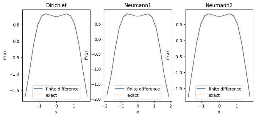
Testing

Here we test our results with the following functions which satisfy the appropriate bondary conditions. (For shorthand we use \(c\) and \(s\) as defined):

(2)\[\begin{align} c &= \cos\frac{2\pi x}{L}, & s &= \sin\frac{2\pi x}{L},\\ f_n(x) &= e^{-ac/2}, & f_n''(x) &= \frac{a\pi^2}{L^2}(as^2 + 2c)f(x),\tag{Neumann}\\ f_d(x) &= e^{-ac/2} - e^{a/2}, & f_d''(x) &= f_n''(x). \tag{Dirichlet} \end{align}\]

def get_f_fixed(x, L, a=1.0, d=0, type='Dirichlet'):
    """Return the d'th derivative of the test function."""
    c = np.cos(2*np.pi*x/L)
    s = np.sin(2*np.pi*x/L)
    f = np.exp(-a*c/2.0)
    df = a*np.pi/L * s * f
    ddf = a*(np.pi/L)**2 * (a*s**2 + 2*c)*f
    if type == 'Dirichlet':
        f -= np.exp(a/2.0)

    if d == 0:
        return f
    elif d == 1:
        return df
    elif d == 2:
        return ddf
    else:
        raise NotImplementedError

L = 4.0
N = 16
plt.figure(figsize=(10,4))
for _n, type in enumerate(['Dirichlet', 'Neumann1', 'Neumann2']):
    plt.subplot(131+_n)
    x, d2 = get_fixed(N=N, L=L, type=(type, type))
    f = get_f_fixed(x, L, d=0, type=type)
    d2f = get_f_fixed(x, L, d=2, type=type)
    plt.plot(x, d2.dot(f), '-', label='finite difference')
    plt.plot(x, d2f, ':', label='exact')
    plt.legend(loc='best')
    plt.xlabel('x')
    plt.ylabel(r"$f''(x)$")
    plt.title(type)

L = 2.0
Ns = 2**np.arange(2, 10)
hs = L / Ns
errs = dict(Dirichlet=[], Neumann1=[], Neumann2=[])

for type in errs:
    for N in Ns:
        x, d2 = get_fixed(N=N, L=L, type=(type, type))
        f = get_f_fixed(x, L, d=0, type=type)
        d2f = get_f_fixed(x, L, d=2, type=type)
        errs[type].append(abs(d2.dot(f) - d2f).max())

# Make errs a numpy array so we can compute with it
for type in errs:
    errs[type] = np.array(errs[type])

# Estimate slope by fitting a polynomial to the two smallest points
fig, ax = plt.subplots()
for type in errs:
    slope, logc = np.polyfit(np.log10(hs[-2:]), np.log10(errs[type][-2:]), 1)
    l = ax.loglog(hs, errs[type], '-+', label=type)[0]
    ax.loglog(hs, 10**logc * hs**2, ':', c=l.get_c(), label=r'$ch^2$')
ax.set_xscale("log", base=2)
ax.legend(loc='best')
ax.set(
    xlabel='$N$',
    ylabel=r"$|f''(x) - D_2\cdot f|$",
    xlim=(hs.min(), hs.max()),
    xticks=hs,
    xticklabels=Ns  # Show N instead of h on bottom axis
)

[Text(0.5, 0, '$N$'),
 Text(0, 0.5, "$|f''(x) - D_2\\cdot f|$"),
 (np.float64(0.00390625), np.float64(0.5)),
 [<matplotlib.axis.XTick at 0x70ccac0c9790>,
  <matplotlib.axis.XTick at 0x70ccac0cbd50>,
  <matplotlib.axis.XTick at 0x70ccac103ad0>,
  <matplotlib.axis.XTick at 0x70ccac105c90>,
  <matplotlib.axis.XTick at 0x70ccac107bd0>,
  <matplotlib.axis.XTick at 0x70ccabf15c90>,
  <matplotlib.axis.XTick at 0x70ccabf17e90>,
  <matplotlib.axis.XTick at 0x70ccabf1e790>],
 [Text(0.5, 0, '4'),
  Text(0.25, 0, '8'),
  Text(0.125, 0, '16'),
  Text(0.0625, 0, '32'),
  Text(0.03125, 0, '64'),
  Text(0.015625, 0, '128'),
  Text(0.0078125, 0, '256'),
  Text(0.00390625, 0, '512')]]

L = 2.2         # Size of box
N = 64          # Number of points

x_p, d2_periodic = get_periodic(N=N, L=L)
x_f, d2_dirichlet = get_fixed(N=N, L=L, type='Dirichlet')
x_f, d2_neumann1 = get_fixed(N=N, L=L, type='Neumann1')
x_f, d2_neumann2 = get_fixed(N=N, L=L, type='Neumann2')

laplacians = [(x_p, d2_periodic, 'Periodic'),
              (x_f, d2_dirichlet, 'Dirichlet'),
              (x_f, d2_neumann1, 'Neumann1'),
              (x_f, d2_neumann2, 'Neumann2')]

Now we plot the first few eigenfunctions (with lowest energy):

fig = plt.figure(figsize=(10, 1))
for _n, (x, d2, label) in enumerate(laplacians):
    Es, Vs = np.linalg.eig(-d2)
    inds = np.argsort(Es)
    Es = Es[inds]
    Vs = Vs[:, inds]
    ax = plt.subplot(141 + _n)
    # Since the sign of the solutions is arbitrary, we normalize
    # by using the sign of the middle point.
    ax.plot(x, Vs[:, :5] / np.sign(Vs[N // 2, :5]))
    ax.set_xlim(-L / 2, L / 2)
    ax.set_xticklabels([])
    ax.set_yticklabels([])
    ax.set_title(label)

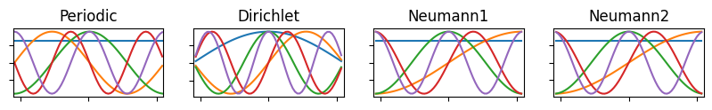
Notice that they obey the correct boundary conditions.

Modes on a drum

Here we present a brute force approach that allows for any shape of drum. The drum shape is specified by a function boundary(x, y) which should return True for all active points on the drum surface.

import matplotlib

L = 2.2
R = 0.9


def drum1(X, Y):
    """Return True for the active points"""
    return X**2 + Y**2 < R**2


def drum1a(X, Y):
    """Return True for the active points"""
    return X**2 + (1.2 * Y)**2 < R**2


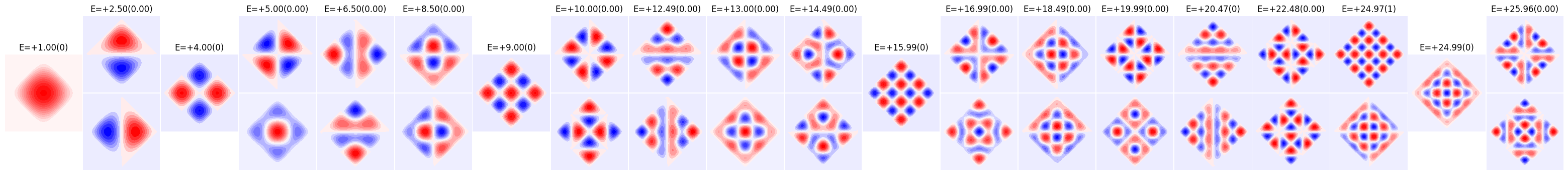
def drum3(X, Y):
    """Return True for the active points"""
    return abs(X) + abs(Y) < R


def drum2(X, Y):
    """Return True for the active points"""
    return np.logical_and(abs(X) < R, abs(Y) < R)


def drum2a(X, Y):
    """Return True for the active points"""
    return np.logical_and(abs(X) < R, abs(1.2 * Y) < R)


def drum2b(X, Y):
    """Return True for the active points"""
    return np.logical_and(abs(X + 0.1 * Y) < R, abs(Y + 0.1 * X) < R)


def drumIa(X, Y):
    """Isospectral drum."""
    Z = 0 * (X + Y)
    c = matplotlib.path.Path([
        (0, 2),
        (1, 3),
        (1, 2),
        (3, 2),
        (3, 1),
        (2, 0),
        (2, 1),
        (1, 1),
    ])
    return c.contains_points(np.array([(X + Z).ravel(),
                                       (Z + Y).ravel()]).T).reshape(Z.shape)


def drumIb(X, Y):
    """Isospectral drum."""
    Z = 0 * (X + Y)
    c = matplotlib.path.Path([
        (0, 2),
        (0, 3),
        (1, 3),
        (1, 2),
        (2, 2),
        (3, 1),
        (2, 1),
        (2, 0),
    ])
    return c.contains_points(np.array([(X + Z).ravel(),
                                       (Z + Y).ravel()]).T).reshape(Z.shape)

Once we have a matrix representation for the second derivative along one dimension, we can form a tensor for the laplacian \(L\):

\[\begin{gather*} L_{ai;bj} = [\mat{D}_2]_{ab}\delta_{ij} + \delta_{ab}[\mat{D}_2]_{ij} \end{gather*}\]

where the indices \(a,b\) act along the \(x\) direction and the indices \(i,j\) act along the \(y\) direction. This type of manipulation is easily performed using the numpy.einsum function which implements the Einstein summation convention.

By grouping the indices as \((ai)\) and \((bj)\) we can reshape the tensor \(L\) into an \(N_xN_y \times N_xN_y\) matrix which we can the use to find the eigenvectors.

To implement the Dirichlet boundary conditions for the drum head, we note that for all points outside of the boundary, \(f_{ai} = 0\), so we can simply remove the corresponding rows and columns from the matrix \(\mat{L}\). Thus completes our strategy for finding the normal modes.

The following code completes basically what is shown in the first TL;DR section of this notebook, but with a bunch of plotting routines to separate out degenerate modes and plot them nicely.

from matplotlib.gridspec import GridSpec, GridSpecFromSubplotSpec
# Need to run /projects/anaconda3/bin/pip install --user uncertainties
from uncertainties import ufloat


def get_periodic(N=64, L=2.2, order=2):
    """Return `(x, d2)` for a periodic box.

    Arguments
    ---------
    N : int
       Number of points
    L : float
       Length of the box

    Returns
    -------
    x : 1d-array
       The abscissa centered in the box.
    d2 : 2d-array
       The laplacian operator in this basis
    """
    h = L / N
    x = np.arange(N) * h - L / 2.0 + h / 2.0
    if order == 2:
        d2 = (-2 * np.eye(N) + np.eye(N, k=1) + np.eye(N, k=-1)) / h**2
        d2[0, -1] = d2[-1, 0] = 1. / h**2
    elif order == 4:
        d2 = -15 * np.eye(N) + 16 * np.eye(N, k=1) - np.eye(N, k=2)
        d2[0, -1] = 16
        d2[1, -1] = d2[0, -2] = -1
        d2 = (d2 + d2.T) / (12.0 * h**2)
    else:
        raise NotImplementedError
    return x, d2


def show_modes(drum,
               levels=20,
               threshold=1e-4,
               degeneracies=None,
               extents=[-1, 1, -1, 1],
               Nxy=(64, 64),
               order=4):

    x0, x1, y0, y1 = extents
    Nx, Ny = Nxy
    Lx, Ly = x1 - x0, y1 - y0
    dx, dy = Lx / Nx, Ly / Ny
    x, d2x = get_periodic(L=Lx, N=Nx, order=order)
    y, d2y = get_periodic(L=Ly, N=Ny, order=order)

    # Center abscissa in extents
    x += Lx / 2 + x0
    y += Ly / 2 + y0

    X, Y = x[:, None], y[None, :]

    D2x = np.einsum('ab,ij->aibj', d2x, np.eye(Ny))
    D2y = np.einsum('ab,ij->iajb', d2y, np.eye(Nx))
    D2 = (D2x + D2y).reshape((Nx * Ny, ) * 2)

    # Get the indices into the 1D ravelled array where the membrane can fluctuate:
    inds = np.where(drum(X, Y).ravel())[0]

    def show(f_, ax):
        f = np.zeros(Nx * Ny)
        f[inds] = f_
        f = f.reshape((Nx, Ny))
        f_ = abs(f).max()
        ax.contourf(x.T, y.T, f.T, 15, cmap='bwr', vmin=-f_, vmax=f_)
        ax.axis('off')
        ax.set(aspect=1)

    # Now restrict the Laplacian to these indices:
    D2_ = D2[inds, :][:, inds]

    # Make sure it is Hermitian
    assert np.allclose(D2_, D2_.T)

    # Find modes
    Es, Vs = np.linalg.eigh(-D2_)

    if degeneracies is None:
        degeneracies = []
        state = 0
        for l in range(levels):
            E0 = Es[state]
            degen = np.sum(abs((Es - E0) / Es[0]) < threshold)
            degeneracies.append(degen)
            state += degen

    vertical = False

    figsize = (2 * max(degeneracies), levels * 2)
    _spec = (levels, 1)
    if not vertical:
        figsize = figsize[::-1]
        _spec = _spec[::-1]

    plt.figure(figsize=figsize)
    gs0 = GridSpec(*_spec, hspace=0.01, wspace=0.01)

    state = 0
    for l, degen in enumerate(degeneracies):
        E0 = Es[state]
        E_ = Es[state:state + degen]
        E = ufloat((E_.max() + E_.min()) / 2, (E_.max() - E_.min()) / 2)
        gs = GridSpecFromSubplotSpec(
            *((1, degen) if vertical else (degen, 1)),
            subplot_spec=gs0[l, 0] if vertical else gs0[0, l],
            hspace=0.01,
            wspace=0.01)
        for _d in range(degen):
            ax = plt.subplot(gs[0, _d] if vertical else gs[_d, 0])
            show(Vs[:, state], ax=ax)
            if _d == 0:
                plt.title("E={:+.2fS}".format(E / Es[0]))
            state += 1
    return degeneracies

Two Iso-spectral Drums

“Can One Hear the Shape of a Drum?” This question dating back to Hermann Wyle was raised by the mathematician Mark Kac [Kac, 1966], and finally answered in [Gordon et al., 1992] who found these two iso-spectral drums. Both have the same spectrum despite having different shapes. Here we generate the eigemode. Differences in the frequencies are due to numerical errors and give one way to assess the accuracy of our approach which we see is accurate at the level of about 2%.

kw = dict(extents=[0, 3, 0, 3], Nxy=(64, 64))
show_modes(drumIa, **kw);
show_modes(drumIb, **kw);

/home/docs/checkouts/readthedocs.org/user_builds/physics-571-math-methods/conda/latest/lib/python3.11/site-packages/uncertainties/core.py:1024: UserWarning: Using UFloat objects with std_dev==0 may give unexpected results.
  warn("Using UFloat objects with std_dev==0 may give unexpected results.")

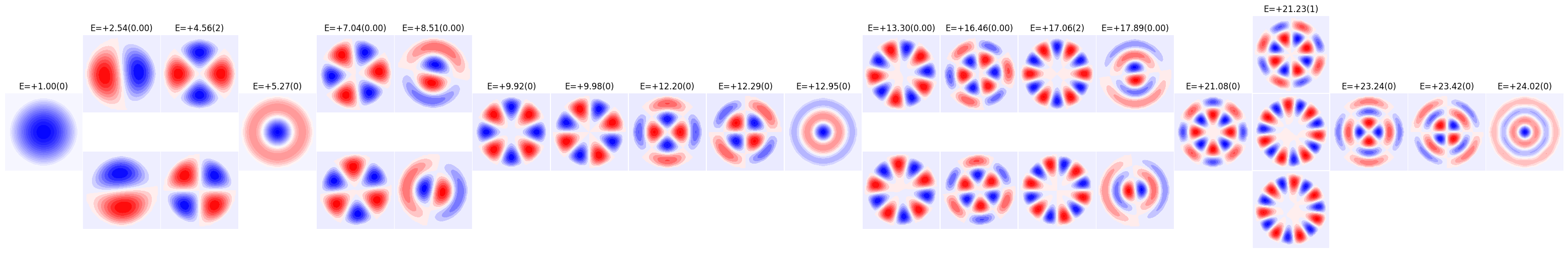
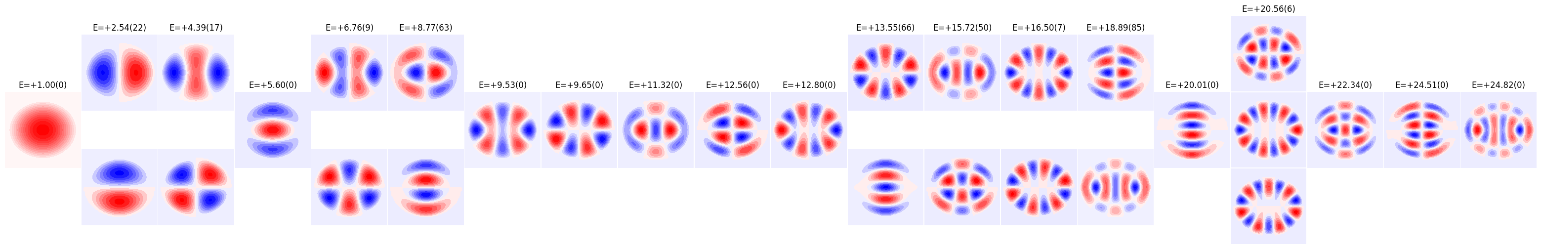
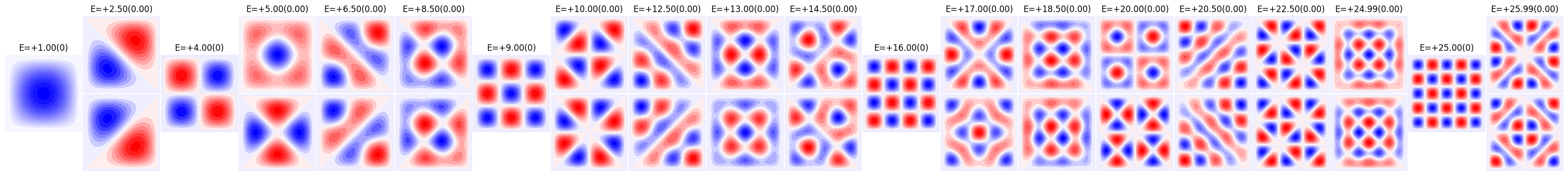
Circular and almost Circular

Here we demonstrate the modes of circular and almost-circular drums. We group these based on their degeneracies. Numerical errors introduce some spurious degeneracies at higher order.

degeneracies = show_modes(drum1, threshold=0.05)
show_modes(drum1a, degeneracies=degeneracies);

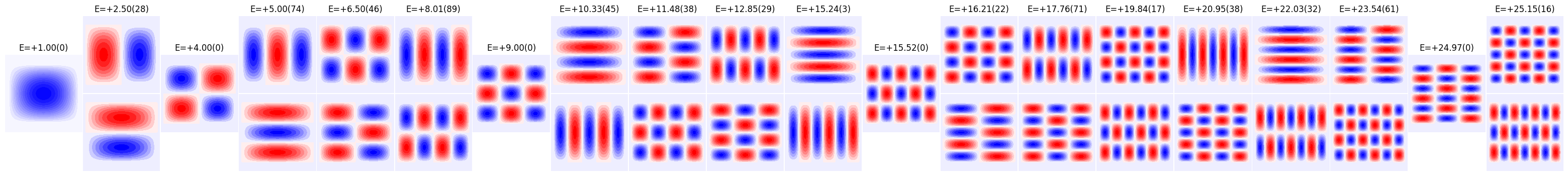
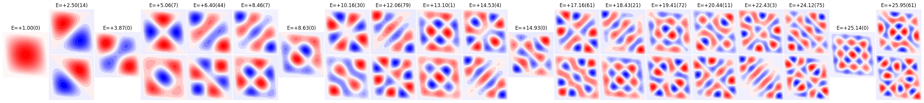
Square and Rectangular

Here are some square and almost square drums. Pure rectangles can be analysed in terms of Fourier modes. The square has degeneracies that numerically end up in some interesting patterns. Different linear combinations would give rise to the “boring” grid patterns seen below for the rectangle which splits the degeneracies. Finally we demonstrate a rotated square which should have the same spectrum as the regular square, but which dhows some different patterns, again due to numerical errors and numerical breaking of the degeneracy.

degeneracies = show_modes(drum2)
show_modes(drum2a, degeneracies=degeneracies)
show_modes(drum2b, degeneracies=degeneracies)
show_modes(drum3, degeneracies=degeneracies);

Analytic Solution

The wave equation

\[\begin{gather*} \nabla^2 \psi - \frac{1}{c^2}\pdiff[2]{}{t}\psi = 0 \end{gather*}\]

is separable in space and time by letting \(\psi(\vect{x}, t) = X(\vect{x})T(t)\). Inserting this and dividing by \(\psi\) we get:

\[\begin{gather*} \frac{\nabla^2 X}{X} = \frac{\frac{1}{c^2}\diff[2]{T}{t}}{T} = -k^2 \end{gather*}\]

where we have chosen the arbitrary constant \(-k^2\) with malice of forethought to emphasize the connection with the wavenumber \(k\). This immediately implies the solution

\[\begin{gather*} T(t) = e^{\I\omega t}, \qquad \omega^2 = c^2k^2. \end{gather*}\]

We next turn to the Helmholtz equation in 2D for \(X(\vect{x})\):

\[\begin{gather*} (\nabla^2 + k^2)X = 0. \end{gather*}\]

This is easy to remember as long as you recall that \(\sqrt{\det\mat{g}}\) plays a role and that it is inside the outer partial:

1. You need an additional factor of \(1/\sqrt{\det\mat{g}}\) outside to keep the dimensions correct.

2. You need to raise the inner index, hence the extra factor of \(g^{\alpha\beta}\).

Recall that, in curvilinear coordinates

\[\begin{gather*} \nabla^2X = \frac{\partial_{\alpha}(\sqrt{\det\mat{g}}\;\partial^{\alpha}X)} {\sqrt{\det\mat{g}}} = \frac{\partial_{\alpha}(\sqrt{\det\mat{g}}\;g^{\alpha\beta}\partial_{\alpha}X)} {\sqrt{\det\mat{g}}}. \end{gather*}\]

For polar coordinates

\[\begin{gather*} \d{s}^2 = \d{r}^2 + r^2\d\phi^2, \qquad \sqrt{\det\mat{g}} = r, \\ g_{\alpha\beta} = \begin{pmatrix} 1\\ & r^2 \end{pmatrix}, \qquad g^{\alpha\beta} = \begin{pmatrix} 1\\ & r^{-2} \end{pmatrix}. \end{gather*}\]

Thus:

\[\begin{gather*} \nabla^2 X = \frac{1}{r}\pdiff{}{r}\left(r\pdiff{X}{r}\right) + \frac{1}{r}\pdiff{\phi}{\phi}\left(r \frac{1}{r^2} \pdiff{X}{\phi}\right) = \frac{1}{r}\pdiff{}{r}\left(r\pdiff{X}{r}\right) + \frac{1}{r^2}\pdiff[2]{X}{\phi}. \end{gather*}\]

It is useful to recognize separability in this form where all of the \(\phi\) dependence occurs in a single term (in the parentheses). Formally you can separate it by solving for

\[\begin{gather*} \frac{\diff[2]{\Phi}{\phi}}{\Phi} = f(r, R). \end{gather*}\]

In this case one could simply multiply through by \(r^2\), but this also works if you have to invert something more complicated.

The Helmholtz equation also separates if we let \(X(\vect{x}) = R(r)\Phi(\phi)\) and divide:

\[\begin{gather*} \frac{\overbrace{\frac{1}{r}\diff{}{r}\left(r\diff{R}{r}\right)} ^{\frac{1}{r^2}\diff[2]{R}{r} + \frac{1}{r}\diff{R}{r}} }{R} + \frac{1}{r^2}\underbrace{\left(\frac{\diff[2]{\Phi}{\phi}}{\Phi}\right)}_{-m^2} = -k^2 \end{gather*}\]

Again, we have chosen the constant \(-m^2\) with malice of forethought – solving gives the following, so we see that \(m\) is an integer:

\[\begin{gather*} \Phi(\phi) = e^{\I m \phi}. \end{gather*}\]

The standard form for the Bessel function is

\[\begin{gather*} x^2\diff[2]{y}{x} + x\diff{y}{x} + (x^2 - m^2)y = 0. \end{gather*}\]

We see that our radial equation has the same form if we multiply through by \(r^2\) and take

\[\begin{gather*} x = kr, \qquad y(x) = R(r). \end{gather*}\]

We can cast the remaining radial equation in the standard form for the Bessel function:

\[\begin{gather*} \diff[2]{R}{r} + \frac{1}{r}\diff{R}{r} + \left(k^2 - \frac{m^2}{r^2}\right)R(r) = 0, \\ x = kr, \qquad R(r)= y(x), \qquad R(r) = \begin{Bmatrix} J_{m}(kr)\\ Y_{m}(kr) \end{Bmatrix}. \end{gather*}\]

Here is a quick and dirty solution for a circular drum head whose analytic solution is

\[\begin{gather*} \psi_{mn}(r, \phi, t) = \Re \left( J_{m}(k_nr) \begin{Bmatrix} e^{\I m\phi}\\ e^{-\I m \phi} \end{Bmatrix} \begin{Bmatrix} e^{\I\omega t}\\ e^{-\I\omega t} \end{Bmatrix} \right), \qquad \omega^2 = k_n^2, \qquad J_m(k_nR) = 0. \end{gather*}\]

Details will be presented below