4. Tensors and Manifolds#
This is my attempt to unify the geometric picture of tensors and manifolds with the practical aspects of “index pushing” needed to do physics. I am attempting to get to the point here, so rigor will be lacking: please see [Hassani, 2013] for careful definitions. This largely replaces the first part of Chapter 4 of [Arfken et al., 2013].
Essential Definitions#
An \(n\)-dimensional (differentiable) manifold \(M\) is a set that every locally looks like Euclidian space \(\mathbb{R}^{n}\). To work with manifolds, we need a collection of charts called an atlas which maps parts of the manifold to subsets of \(\mathbb{R}^{n}\).
For the purposes of this discussion, we will consider manifolds that are embedded in a higher dimensional Euclidian space \(M\subset \mathbb{R}^{m}\). This embedding will allow use to determine the metric \(\op{g}\), but it is not necessary that manifolds be embedded (or even that they can be embedded, though most can). These manifolds are call Riemannian manifolds.
Important
All of the information about the nature of the manifold is contained in the metric \(\op{g}\). Thus: even if we don’t have (or know) the embedding, we can still work with the manifold if we know \(\op{g}\).
We will start with embedded manifolds, but once we develop the formalism, we will be able to describe, e.g., spacetime, where we cannot “get out” to see the embedding. For example, consider a sphere like the surface of the earth. From space we can see that the surface is curved, and we can calculate anything we like using Euclidian geometry, but as people living on the earth, we must infer properties like the curvature by making local measurements within the manifold itself.
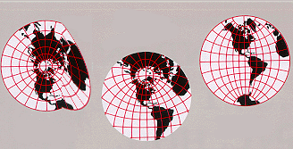
Fig. 1 Example of different charts for describing the surface of the earth – an \(m=2\)-dimensional manifold embedded in \(n=3\)-dimensional space \(\mathbb{R}^3\).#
Embedded Manifolds#
To be concrete, we start with an embedded \(m\)-dimensional manifold \(M\subset \mathbb{R}^{n}\) where \(n\geq m\). This allows us to use Cartesian coordinates \(x \in \mathbb{R}^{n}\) to describe points on the manifold. To work on the manifold, however, we would like to use a different set of coordinates \(X \in \mathbb{R}^{m}\).
Notation
Since there are \(m\) coordinates \(X^{\alpha}\), it is tempting to use the notation \(\vect{X}\) to describe the points. I will try to refrain from doing this, however, since these points are not vectors in the sense of the manifold – it make no sense to “add” two points on a sphere for example. Instead I will just use \(x\) and \(X\) to represent these, and reserve vector notation for the vector spaces like the tangent space.
For the actual vectors and covectors I will use bra-ket notation:
where \(\{\ket{X_\alpha}\}\) is a set of basis vectors and \(\{\bra{X^\alpha}\}\) is a basis of covectors (forms). Here an everywhere unless explicitly stated otherwise, we will use the Einstein summation convention of summing over repeated indices.
In this discussion, we will consider primarily two sets of coordinates: Euclidean coordinates in the embedding space \(x^{i}\), and general coordinates in the chart \(X^{\alpha}\). To help distinguish between these, we will use lower-case letters \(x\) and latin indices \(i\), \(j\), \(k\), \(l\), etc. for the Euclidean coordinates, and upper case letters \(X\) with greek indices \(\alpha\), \(\beta\), \(\gamma\), \(\delta\) etc. for the chart coordinates \(X^{\alpha}\). This choice is so that the usual Euclidean coordinates \(x^1\), \(x^2\) look familiar.
To describe the manifold, we can define the \(n\) functions
Working Example: Polar coordinates
To keep things straight, I recommend thinking about polar coordinates on the unit sphere:
Note that it is natural to express \(x^{i}(X^{\alpha})\) since this is an embedding: Use this as the basis for the Jacobian \(J^{i}{}_{\alpha} = \partial x^{i}/\partial X^{\alpha}\). Conversely, it is somewhat unnatural to express the inverse \(X^{\alpha}(x^{i})\) which is not uniquely defined.
This provides a complete description of the manifold and its properties everywhere these functions are not singular.
Concrete Examples: Polar coordinates and a unit sphere
To keep things real, we will follow two concrete examples:
Polar coordinates for describing the plane \(\mathbb{R}^2\) with \(m=n=2\).
Here \((x^1, x^2) = (x, y)\) and \((X^1, X^2) = (r, \phi)\):
\[\begin{align*} x^1(X^1, X^2) &= x(r, \phi) = r\cos\phi = X^1 \cos X^2,\\ x^2(X^1, X^2) &= y(r, \phi) = r\sin\phi = X^1 \sin X^2. \end{align*}\]Inverting these
\[\begin{align*} X^1(x^1, x^2) &= r(x, y) = \sqrt{(x)^2 + (y)^2} = \sqrt{(x^1)^2 + (x^2)^2},\\ X^2(x^1, x^2) &= \phi(x, y) = \tan^{-1}\frac{y}{x} = \tan^{-1}\frac{x^2}{x^1}. \end{align*}\]Unit sphere: Spherical coordinates for describing points on the surface of the unit sphere with \(m=2\) embedded in \(n=3\).
Here \((x^1, x^2, x^3) = (x, y, z)\) and \((X^1, X^2) = (\theta, \phi)\):
\[\begin{align*} x^1(X^1, X^2) &= x(\theta, \phi) = \sin\theta\cos\phi = \sin X^1 \cos X^2,\\ x^2(X^1, X^2) &= y(\theta, \phi) = \sin\theta\sin\phi = \sin X^1 \sin X^2,\\ x^3(X^1, X^2) &= z(\theta, \phi) = \cos\theta = \cos X^1. \end{align*}\]Inverting these
\[\begin{align*} X^1(x^1, x^2, x^3) &= \theta(x, y, z) = \cos^{-1}z = \cos^{-1}x^3,\\ X^2(x^1, x^2, x^3) &= \phi(x, y, z) = \tan^{-1}\frac{y}{x} = \tan^{-1}\frac{x^2}{x^1}. \end{align*}\]Restricted to the sphere:
\[\begin{gather*} x^2 + y^2 + z^2 = 1,\\ x^2 + y^2 = 1 - z^2 = 1-\cos^2\theta = \sin^2\theta. \end{gather*}\]
Note that neither of these charts is sufficient to fully describe the full manifold since they are singular at e.g. \(r=0\) and \(\theta = 0\). The spherical chart is also not properly differentiable at the boundaries – i.e. physically the points \(\phi\) and \(\phi+2\pi\) should be identified, but according to the chart, they are different.
We will restrict our attention to a submanifold that is simply connected and has no singularities for this discussion.
Jacobian Matrix#
In particular, properties of the embedding space can be converted to properties of the manifold through the Jacobian matrix \(\mat{J}\) and its inverse \(\mat{J}^{-1}\):
Note that if we think of \(x^i = f(X)\) as a vector valued function, then \(\mat{J} = \mat{\d} f\) is the differential such that
In matrix form:
Note that \(\mat{J}^{-1}\mat{J} = \mat{1}\), but that \(\mat{J}\mat{J}^{-1}\) may be rank deficient if \(m < n\).
Concrete Examples: Polar coordinates and a unit sphere
Polar coordinates:
\[\begin{gather*} \mat{J} = \pdiff{(x, y)}{(r, \phi)} =\begin{pmatrix} \cos\phi & -r\sin\phi \\ \sin\phi & r\cos\phi \end{pmatrix}, \\ \mat{J}^{-1} = \pdiff{(r, \phi)}{(x, y)} = \begin{pmatrix} x/r & y/r \\ x/r^2 & -y/r^2 \end{pmatrix} = \begin{pmatrix} \cos\phi & \sin\phi \\ r^{-1}\cos\phi & -r^{-1}\sin\phi \end{pmatrix} \end{gather*}\]Notice that \(\mat{J}^{-1}\mat{J} = \mat{J}\mat{J}^{-1} = \mat{1}\), justifying the nomenclature.
Unit sphere:
\[\begin{gather*} \mat{J} = \pdiff{(x, y, z)}{(\theta, \phi)} = \begin{pmatrix} \cos\theta\cos\phi & -\sin\theta\sin\phi \\ \cos\theta \sin\phi & \sin\theta\cos\phi \\ -\sin\theta & 0 \end{pmatrix},\\ \mat{J}^{-1} = \pdiff{(\theta, \phi)}{(x, y, z)} = \begin{pmatrix} 0 & 0 & \frac{-1}{\sqrt{1 - z^2}}\\ \frac{-y}{x^2+y^2} & \frac{x}{x^2+y^2} & 0 \end{pmatrix} = \begin{pmatrix} 0 & 0 & \frac{-1}{\sin\theta}\\ \frac{-\sin\phi}{\sin\theta} & \frac{\cos\phi}{\sin\theta} & 0 \end{pmatrix}. \end{gather*}\]\[\begin{gather*} \mat{J}\mat{J}^{-1} = \begin{pmatrix} \sin^2\phi & - \sin\phi\cos\phi & -\cot\theta \cos\phi \\ -\sin\phi\cos\phi & \cos^2\phi & -\cot\theta\sin\phi\\ 0 & 0 & 1 \end{pmatrix}. \end{gather*}\]Within the manifold, \(\mat{J}^{-1}\mat{J} = \mat{1}\), but within the embedded space, \(\mat{J}\mat{J}^{-1} \neq \mat{1}\) since the Jacobian matrix is rank deficient.
Vectors#
Consider a particle moving on the manifold. This motion can be described by the curve with coordinates \(x\bigl(X(t)\bigr)\) through the embedded space. This curve defines the velocity vector \(\ket{v}\):
Note: the vector \(\ket{v}\) represents a “physical” object – something real (as defined by the embedding). By contrast, the components \(v^{i}\) and \(V^{\alpha}\) are the “columns of numbers” often associated with vectors.
Unlike the actual vector \(\ket{v}\), these numbers depend on the coordinate choice.
Comparison with notation in [Arfken et al., 2013]
Remember that here we use \(v^{i}\) as the components of the vector \(\ket{v}\) in Euclidean embedding space, and \(V^{\alpha}\) as the coefficients in the chart. We are relying on the type of indices to distinguish. In contrast, [Arfken et al., 2013] use a prime. Thus, we have
[Arfken et al., 2013] also uses \(\boldsymbol{\varepsilon}^i\) which would correspond to \(\ket{X^{\alpha}}=\ket{X_{\beta}}g^{\beta\alpha}\). One can in principle use these, but we instead express everything in the natural form where basis vectors always have lower indices. In our notations \(\ket{X^{\alpha}}\) or \(\bra{X_{\alpha}}\) would probably indicate we have made a mistake. See e.g. our comment about (4.50).
The Jacobian matrix \(\mat{J}\) plays two roles here:
Acting to the right, it transforms the components of a vector in the chart \(V^{\alpha}\) into the coordinates in the embedding space \(v^i\). Acting to the left, (or equivalently, the transpose \(\mat{J}^T\) acting to the right), it transforms the basis vectors \(\ket{\hat{e}_i}\) from the embedding space into the coordinate basis vectors \(\ket{X_\alpha}\) that we can use to express vectors like the velocity in terms of its components \(V^{\alpha} = \dot{X}^\alpha\) in the chart coordinates.
Important
The basis vectors \(\ket{X_\alpha}\) need not be orthonormal in the embedding space. It is often convenient to choose coordinates where the basis is at least orthogonal as this makes the metric nice, but it is not necessary or assumed here.
However, the basis vectors are orthonormal in the sense that \(\braket{X^\alpha|X_\beta}=\delta^{\alpha}_{\beta}\). In fact, as we shall see, the metric is exactly the thing that allows us to define such an inner product, and is precisely defines so that these basis vectors remain orthonormal.
We are being careful about our index location. The components of the contravariant vectors are expressed with an upper index: \(V^{\alpha}\) (expressed in the chart) and \(v^{i}\) (expressed in the embedding space). To keep the index convention, we label the actual basis vectors with a lower index \(\ket{X_{\alpha}}\).
Concrete Examples: Polar coordinates and a unit sphere
Polar coordinates:
\[\begin{gather*} \begin{pmatrix} \ket{r} & \ket{\phi} \end{pmatrix} = \begin{pmatrix} \ket{\hat{x}} & \ket{\hat{y}} \end{pmatrix} \underbrace{ \begin{pmatrix} \cos\phi & -r\sin\phi\\ \sin\phi & r\cos\phi \end{pmatrix}}_{\mat{J}}\\ \ket{r} = \ket{\hat{x}}\cos\phi + \ket{\hat{y}}\sin\phi, \\ \ket{\phi} = -\ket{\hat{x}}r\sin\phi +\ket{\hat{y}}r\cos\phi. \end{gather*}\]Unit sphere:
\[\begin{gather*} \begin{pmatrix} \ket{\theta} & \ket{\phi} \end{pmatrix} = \begin{pmatrix} \ket{\hat{x}} & \ket{\hat{y}} & \ket{\hat{z}} \end{pmatrix} \underbrace{ \begin{pmatrix} \cos\theta\cos\phi & -\sin\theta\sin\phi\\ \cos\theta\sin\phi & \sin\theta\cos\phi\\ -\sin\theta & 0 \end{pmatrix}}_{\mat{J}}\\ \ket{\theta} = \ket{\hat{x}}\cos\theta\cos\phi + \ket{\hat{y}}\cos\theta\sin\phi - \ket{\hat{z}}\sin\theta, \\ \ket{\phi} = -\ket{\hat{x}}\sin\theta\sin\phi + \ket{\hat{y}}\sin\theta\cos\phi. \end{gather*}\]

Fig. 2 Visual depiction of a vector \(\ket{a}\) (top) and a covector \(\bra{v}\) (middle). The bottom shows the covector \(\bra{v}\) acting on the vector \(\ket{a}\) to give \(\braket{v|a} = 2\). Notice that the vector would pierce the stacked covector exactly two times.#
Covectors (Forms)#
In addition to vectors, we also have covectors or 1-forms: these are linear operators which take vectors into numbers, and should be thought of as the manifold generalization of row vectors \(\bra{v}\):
Given a basis of covectors \(\{\bra{X^{\alpha}}\}\), we can express a covector \(\bra{v}\) as
Here we use lower indices for the coefficients \(V_\alpha\) which called covariant in contradistinction to the contravariant \(V^\alpha\) with raised indices that describe the vector (or contravariant vector) \(\ket{v}\):
Important
Without a metric, there is no way to relate vectors and covectors. Geometrically they are different types of objects. (See Fig. 2.) Thus, the contravariant coefficients \(V^{\alpha}\) of the vector bear no relationship with the covariant coefficients \(V_\alpha\) of the covector.
We can choose the basis of covectors \(\{\bra{X^{\alpha}}\}\) to be dual to the basis of vectors \(\{\ket{X_{\alpha}}\}\):
For this to be invariant under coordinate transforms, the covariant coefficients \(V_{\alpha}\) and dual basis vectors must transform with the inverse Jacobian \(\mat{J}^{-1}\):
Concrete Examples: Polar coordinates and a unit sphere
Polar coordinates:
\[\begin{gather*} \begin{pmatrix} \bra{r}\\ \bra{\phi} \end{pmatrix} = \underbrace{ \begin{pmatrix} \cos\phi & \sin\phi\\ r^{-1}\cos\phi & -r^{-1}\sin\phi \end{pmatrix}}_{\mat{J}^{-1}} \begin{pmatrix} \bra{\hat{x}}\\ \bra{\hat{y}} \end{pmatrix}\\ \begin{aligned} \bra{r} &= \cos\phi\bra{\hat{x}} + \sin\phi\ket{\hat{y}}, \\ \bra{\phi} &= r^{-1}\cos\phi\bra{\hat{x}} - r^{-1}\sin\phi\bra{\hat{y}}. \end{aligned} \end{gather*}\]Unit sphere:
\[\begin{gather*} \begin{pmatrix} \bra{\theta}\\ \bra{\phi} \end{pmatrix} = \underbrace{ \begin{pmatrix} 0 & 0 & \frac{-1}{\sin\theta}\\ \frac{-\sin\phi}{\sin\theta} & \frac{\cos\phi}{\sin\theta} & 0 \end{pmatrix}}_{\mat{J}^{-1}} \begin{pmatrix} \bra{\hat{x}}\\ \bra{\hat{y}}\\ \bra{\hat{z}} \end{pmatrix},\\ \begin{aligned} \bra{\theta} &= \frac{-\bra{\hat{z}}}{\sin\theta},\\ \bra{\phi} &= \frac{-\sin\phi\bra{\hat{x}} + \cos\phi\bra{\hat{y}}}{\sin\theta}. \end{aligned} \end{gather*}\]
Completeness#
Armed with these dual bases, we can express the identity operator as
Transformations#
The key property of vectors and covectors, and the defining properties of tensors, is that their components transform linearly under coordinate transformation:
Invariance of the action of forms on vectors implies
In matrix form:
Linearity
To see that vectors transform linearly, consider two set of coordinates \(X^{\alpha}(x)\) and \(\tilde{X}^{\alpha}(x)\) as functions of the same embedding space
Thus, \(\mat{\Gamma}\) is just the Jacobian \(\mat{J}\) for the transformation between the two coordinates \(X(\tilde{X})\). Thus, this is linear even if the coordinate transformations are non-linear.
If you have a collection of numbers that does not transform appropriately, then it cannot be considered to be a tensor.
Tensors#
Let \(\mathcal{V}\) denote a vector space (i.e., the space of tangent vectors at a fixed point in the manifold), and let \(\mathcal{V}^*\) denote the dual space of covectors. A tensor \(\op{T}^{r}_{s}\) in \(\mathcal{T}^{r}_{s}(\mathcal{V})\) on \(\mathcal{V}\) is a multilinear map
Thus, covectors are tensors in \(\mathcal{T}_{1}^{0}(\mathcal{V})\) since they take vectors into numbers, and vectors are tensors in \(\mathcal{T}^{1}_{0}(\mathcal{V})\) since they take covectors into numbers. Given a basis \(\ket{X_{\alpha}}\) for \(\mathcal{V}\) and a basis \(\bra{X^{\alpha}}\) for \(\mathcal{V}^*\), the components of the tensor are
and we can write
Metric Tensor#
A metric tensor (or metric) \(\op{g}\in \mathcal{T}^{0}_{2}(\mathcal{V})\) acts as an inner product on the vector space: it is bilinear operation that takes two vectors into a real number, satisfying all of the properties of an inner product (a.k.a. dot product):
Thus, given a vector \(\ket{v}\), the metric defines a linear operator that acts on vectors returning numbers. In other words, it maps the vector \(\ket{v}\) to a covector \(\bra{v}\):
Note that the metric may be different at different points in the manifold: thus we should think of metric tensor field. If the manifold is not embedded in another space, then the metric provides all of the information about the manifold’s structure.
If the manifold is embedded, however, then we can use the Jacobian matrix \(\mat{J}\) to induce the metric from the embedding because the embedding space \(\mathbb{R}^n\) has a nature metric – the Euclidean metric – which we can use to induce the metric on the manifold.
Consider the dot product of two vectors \(\ket{a}\) and \(\ket{b}\):
The inner product can now be induced from the embedding space:
Note that the metric in the embedding space is just the identity \(\delta_{ij}\), so the covariant components equal the contravariant components: \(a_i = a^i\). This is generally not true in the chart \(A_\alpha \neq A^\alpha\). Equating the inner product in the chart and the embedding space, we have
Thus, we have
Note that \(g_{\alpha\beta} = g_{\beta\alpha}\) is symmetric.
Stated more directly
Armed with these coefficients, we can compute the covariant coefficients \(A_\alpha\):
where we say that the metric lowers the index. Note that these are the coefficients of the covector \(\bra{a}\):
With this notation, we can write the contraction
It is also useful to define a related set of numbers \(g^{\alpha\beta}\) which raise the index, taking covariant components back into contravariant components:
This must be the matrix inverse of \(g_{\alpha\beta}\):
Notation of [Arfken et al., 2013]
[Arfken et al., 2013] uses the notation
and writes the calculation of \(g_{ij}\) as
In our notation, we would write this in terms of the transpose \(\bra{X_\alpha} = \ket{X_\alpha}^T\):
Note that the transpose is not the same as the dual:
As this suggests, the duals are formed using the metric:
[Arfken et al., 2013] defines
This is equivalent to our notation:
Concrete Examples: Polar coordinates and a unit sphere
Polar coordinates:
\[\begin{align*} \mat{g} &= \mat{J}^T\mat{J} = \begin{pmatrix} \cos\phi & \sin\phi \\ -r\sin\phi & r\cos\phi \end{pmatrix} \begin{pmatrix} \cos\phi & -r\sin\phi \\ \sin\phi & r\cos\phi \end{pmatrix}\\ &= \begin{pmatrix} \cos^2\phi + \sin^2\phi & 0 \\ 0 & r^2(\cos^2\phi + \sin^2\phi) \end{pmatrix}\\ &= \begin{pmatrix} 1 & 0 \\ 0 & r^2 \end{pmatrix}. \end{align*}\]Unit sphere:
\[\begin{align*} \mat{g} &= \mat{J}^T\mat{J} \\ &= \begin{pmatrix} \cos\theta\cos\phi & \cos\theta \sin\phi & -\sin\theta\\ -\sin\theta\sin\phi & \sin\theta\cos\phi & 0 \end{pmatrix} \begin{pmatrix} \cos\theta\cos\phi & -\sin\theta\sin\phi \\ \cos\theta \sin\phi & \sin\theta\cos\phi \\ -\sin\theta & 0 \end{pmatrix}\\ &= \begin{pmatrix} \cos^2\theta\cos^2\phi + \cos^2\theta \sin^2\phi +\sin^2\theta & 0\\ 0 & \sin^2\theta\sin^2\phi + \sin^2\theta\cos^2\phi \end{pmatrix}\\ &= \begin{pmatrix} 1 & 0\\ 0 & \sin^2\theta \end{pmatrix}. \end{align*}\]
“The Metric” (Geodesics)#
How do we relate the metric tensor \(\op{g}\) with the idea of a metric that allows us to compute distances? This is expressed in terms of the line element \(\d{s}\):
One can then integrate a curve to obtain the distance between two points
A geodesic is a path \(\gamma(s)\) that minimizes the distance between two points. Using calculus of variations, we can derive the geodesic equations satisfied by such a path (see below).
Concrete Examples: Polar coordinates and a unit sphere
Polar coordinates:
\[\begin{gather*} \d{s}^2 = \d{x}^2 + \d{y}^2 = \d{r}^2 + r^2\;\d{\phi}^2. \end{gather*}\]Unit sphere:
\[\begin{gather*} \d{s}^2 = \d{\theta}^2 + \sin^2\theta\;\d{\phi}^2. \end{gather*}\]
Derivatives#
Complications arrive in the notion of derivatives because, by their nature, they compare the behavior of vectors in different spaces – at neighboring points. In the Euclidean embedded space, this is not an issue since all vectors live in the same space, but once we introduce coordinate transforms, there is no guarantee about how the tangent space at neighboring points are related.
Important
The idea of covariance is we consider only quantities that are well defined within the manifold, or embedding space. For example, we can consider quantities like the number returned by a form acting on a vector \(\braket{u|v}\) or the number returned by the metric \(\op{g}\bigl(\ket{u}, \ket{v}\bigr)\) (which is the same if the space has a metric to related \(\ket{u}\) and \(\bra{u}\).) These values should not change if we change our coordinate system: in other words, they are invariant under coordinate transformations.
In contrast, the “numbers” like \(V^{\alpha}\), which are the components of the vector in a particular chart, depend on the choice of coordinates – specifically through the Jacobian matrix \(J_{\alpha}{}^{i} = \partial_{\alpha}x^{i}\). Since physicists like to work with numbers, much attention is given to these coordinates, and how they transform – so much so that some books refer to the numbers themselves as tensors. The emphasis on how the components transform is so that physicists can ensure that they are forming invariant quantities by contracting indices in covariant-contravariant pairs: \(\braket{u|v} = U_{\alpha}V^{\alpha}\).
To ensure that you are studying physics rather than numerology, I recommend that you try to express all of your final results in terms of fundamental properties of the manifold – or at least in terms of properties computed in the embedding space. Of course, work with coordinates because they are useful, but don’t trust that something is coordinate invariant just because the indices are properly paired – make sure you understand what the quantity means physically.
To see how one might get into difficulty, consider a function \(f(x)\) on the manifold where \(x(X)\) depend on some chart coordinates \(X\). The gradient in the coordinate chart is
We thus see that that coefficients of the gradient behave naturally as a covector
Notation
This motivates the following notation to emphasize the covariant nature of derivatives.
We will use this notation going forward:
We can now consider various derivative operations constructed from
Unless specified otherwise, the derivative should act to the right.
Warning
If you carefully use \(\bra{\nabla}\) and \(\ket{\nabla}\) as we do below, you will obtain properly invariant quantities, but you can run into difficulty if you blindly use \(\partial_{\alpha}\). For example, you might think that
are the components of a tensor in \(\mathcal{T}^{1}_{1}\), but it is not. In particular,
is not the proper divergence in general, and is not invariant under coordinate transforms.
Example in Polar Coordinates
Consider the vector field \(\ket{v} = \ket{x}x + \ket{y}y\) with divergence \(\braket{\nabla|v} = 1\). In polar coordinates \(x+\I y = r^{\I\phi}\) we have
hence
This only gives the correct answer along the \(x\)-axis.
Christoffel Symbols#
In general, the basis vectors \(\ket{X_j}\) for the chart might change as one moves along the manifold. This change can re-expressed in terms of the basis:
The coefficient \([\alpha\beta,\gamma]\) are known as the Christoffel symbols of the first kind and \(\Gamma^{\gamma}_{\alpha\beta}\) are known as the Christoffel symbols of the second kind. They can be computed by differentiating the basis vectors:
These formulae should make it clear that, for the tangent space, \(\Gamma^{\gamma}_{\alpha\beta} = \Gamma^{\gamma}_{\beta\alpha}\) is symmetric in the lower indices.
Important
Although we use index notation, \(\Gamma\) is not a tensor. To see this, note that in Euclidean coordinates, \(g_{ij} = \delta_{ij}\) is constant, so \(\Gamma^{\gamma}_{\alpha\beta} = 0\). If this were to transform as a tensor by multipliction with Jacobian factors, then it would have to be zero in all frames, which is clearly not.
Exercise: Compute the Christoffel symbols.
These are obtained by differentiating the basis vectors:
Notice that these are symmetric in \(\alpha\) and \(\beta\):
Can we express this in terms of the metric?
This looks promising, but we need to cancel some terms. Consider two other permutations permutations:
This should make it clear that
Concrete Examples: Polar coordinates and a unit sphere
Since the metric in both cases is simple, we use the metric formulae. To obtain a non-zero entry for \([\alpha\beta,\gamma]\) we need one of \(\beta=\gamma\), \(\alpha=\gamma\), or \(\alpha=\beta\). We can also use the symmetry \([\alpha\beta,\gamma]=[\beta\alpha,\gamma]\):
Polar coordinates:
Since \(g_{rr} = 1\) and \(g_{\phi\phi} = r^2\), the only non-zero contribution will be from
\[\begin{gather*} \pdiff{g_{\phi\phi}}{X_r} = \pdiff{r^2}{r} = 2r. \end{gather*}\]This requires one of \((\alpha, \beta, \gamma) \in \{(r, \phi, \phi), (\phi, r, \phi), (\phi, \phi, r)\}\):
\[\begin{gather*} [r\phi,\phi] = [\phi r,\phi] = - [\phi\phi,r] = r,\\ \Gamma^{\phi}_{r\phi} = \Gamma^{\phi}_{\phi r} = \frac{1}{r}, \qquad \Gamma^{r}_{\phi\phi} = -r. \end{gather*}\]Geometrically this makes sense: If we increase \(r\), the basis vectors do not rotate, but \(\ket{\phi}\) will change length, whereas if we increase \(\phi\), they both rotate. The basis vectors are
\[\begin{align*} \partial_{\phi}\ket{r} &= -\ket{\hat{x}}\sin\phi + \ket{\hat{y}}\cos\phi = \frac{1}{r}\ket{\phi} = \ket{\phi}\Gamma^{\phi}_{r\phi},\\ \partial_{r}\ket{\phi} &= \frac{1}{r}\ket{\phi} = \ket{\phi}\Gamma^{\phi}_{\phi r}, \\ \partial_{\phi}\ket{\phi} &= -\ket{\hat{x}}r\cos\phi - \ket{\hat{y}}r\sin\phi = -r\ket{r} = \ket{r}\Gamma^{r}_{\phi\phi}. \end{align*}\]Unit sphere:
Here we will compute these directly from the basis vectors:
\[\begin{gather*} \ket{\theta} = \ket{\hat{x}}\cos\theta\cos\phi + \ket{\hat{y}}\cos\theta\sin\phi - \ket{\hat{z}}\sin\theta, \\ \ket{\phi} = -\ket{\hat{x}}\sin\theta\sin\phi + \ket{\hat{y}}\sin\theta\cos\phi. \end{gather*}\]\[\begin{align*} \partial_{\theta}\ket{\theta} &= -\ket{\hat{x}}\sin\theta\cos\phi - \ket{\hat{y}}\sin\theta\sin\phi - \ket{\hat{z}}\cos\theta = \cot\theta \ket{\theta} + -\ket{\hat{x}}\cos\phi/\sin\theta -\ket{\hat{y}}\sin\phi/\sin\theta ,\\ \partial_{\phi}\ket{\theta} &= -\ket{\hat{x}}\cos\theta\sin\phi + \ket{\hat{y}}\cos\theta\cos\phi = \ket{\phi}\cot\theta = \ket{\phi}\Gamma^{\phi}_{\theta\theta},\\ \partial_{\theta}\ket{\phi} &= -\ket{\hat{x}}\cos\theta\sin\phi + \ket{\hat{y}}\cos\theta\cos\phi = \ket{\phi}\cot\theta = \ket{\phi}\Gamma^{\phi}_{\phi\theta},\\ \partial_{\phi}\ket{\phi} &= -\ket{\hat{x}}\sin\theta\cos\phi -\ket{\hat{y}}\sin\theta\sin\phi,\\ \end{align*}\]The structure is the same, but now we have
\[\begin{gather*} \pdiff{g_{22}}{X_1} = \pdiff{\sin^2\theta}{\theta} = 2\sin\theta \cos \theta = \sin(2\theta). \end{gather*}\]\[\begin{gather*} [12,2] = [21,2] = - [22,1] = \frac{\sin(2\theta)}{2},\\ \Gamma^{2}_{12} = \Gamma^{2}_{21} = \frac{\sin(2\theta)}{2\sin^2\theta} = \cot\theta, \qquad \Gamma^{1}_{22} = -\frac{\sin(2\theta)}{2}. \end{gather*}\]Stated more nicely:
\[\begin{gather*} [\theta\phi,\phi] = [\phi\theta,\phi] = - [\phi\phi,\theta] = \sin\theta\cos\theta,\\ \Gamma^{\phi}_{\theta\phi} = \Gamma^{\phi}_{\phi \theta} = \cot\theta, \qquad \Gamma^{\theta}_{\phi\phi} = -\sin\theta\cos\theta \end{gather*}\]We can check by direct differentiation:
\[\begin{gather*} (x, y, z) = (\sin\theta\cos\phi, \sin\theta\sin\phi, \cos\theta)\\ [\theta\phi,\phi] = \pdiff{x^i}{\phi}\frac{\partial^2 x^i}{\partial\phi\partial\theta} = \pdiff{x}{\phi}\frac{\partial^2 x}{\partial\phi\partial\theta} + \pdiff{y}{\phi}\frac{\partial^2 y}{\partial\phi\partial\theta}\\ = -\sin\theta\sin\phi(-\cos\theta\sin\phi) + \sin\theta\cos\phi(\cos\theta\cos\phi) = \sin\theta\cos\theta,\\ [\phi\phi,\theta] = \pdiff{x^i}{\theta}\pdiff[2]{x^i}{\phi} = \pdiff{x}{\theta}\pdiff[2]{x}{\phi} + \pdiff{y}{\theta}\pdiff[2]{y}{\phi}\\ = \cos\theta\cos\phi(-\sin\theta\cos\phi) + \cos\theta\sin\phi(-\sin\theta\sin\phi) = -\sin\theta\cos\theta. \end{gather*}\]
The case of a Diagonal Metric
If the metric is diagonal, then we have many simplifications. For example:
Recalling that \(h^{\gamma} = 1/h_{\gamma}\) one can use this to show that, at least for diagonal metrics
which is generally true.
Geodesics#
The geodesic equations can be found by minimizing the “energy” functional
where \(\gamma(t)\) is a path from \(a\) and \(b\) whose parameterization is chosen so that the speed is constant over the whole path:
where \(L(\gamma)\) is the length of the path. Recall that the path is described by the coordinates \(X^i(t)\), so
The energy can be minimized using calculus of variations, and which gives the geodesic equation
The same Christoffel symbols (of the second kind) enter.
Gradient#
The gradient of a function is straightforward:
Note that this is naturally a form (covector) since the gradient of a function takes a vector (curve) and computes the directional derivative of the function along that direction:
Furthermore, note that, for this to be invariant, the gradient must act as a covariant tensor, hence justifying the compact notation with a lower index.
Covariant Derivative#
Differentiating a vector \(\ket{v} = \ket{X_\alpha}V^{\alpha}\) is more complicated because the basis elements may also change, as described by the Christoffel symbols. We start by considering the following, where the where the derivative acts to the left:
Inserting the identity \(\op{1} = \ket{X_\alpha}\bra{X^{\alpha}}\) we recover the Christoffel symbols:
This is the covariant derivative of a vector:
Unlike \(\partial_{\beta}V^{\alpha} \equiv V^{\alpha}_{,\beta}\), this transforms properly and deserves the shorthand notation.
Divergence#
We can also act the form on the vector to obtain the divergence:
The contraction on the two indices of the Christoffel symbol has a nice form in terms of the determinant of the metric
where \(\det(g)\) is the determinant of \(g_{\alpha\beta}\):
Laplacian#
Finally, the Laplacian can be computed by taking the divergence of the gradient after first using inverse metric to convert the gradient to a vector:
Expanded fully, this gives: