Show code cell content

Hide code cell content

import mmf_setup

mmf_setup.nbinit()
import logging

logging.getLogger("matplotlib").setLevel(logging.CRITICAL)
%matplotlib inline
import numpy as np, matplotlib.pyplot as plt

$\newcommand{\vect}[1]{\mathbf{#1}} \newcommand{\uvect}[1]{\hat{#1}} \newcommand{\abs}[1]{\lvert#1\rvert} \newcommand{\norm}[1]{\lVert#1\rVert} \newcommand{\I}{\mathrm{i}} \newcommand{\ket}[1]{\left|#1\right\rangle} \newcommand{\bra}[1]{\left\langle#1\right|} \newcommand{\braket}[1]{\langle#1\rangle} \newcommand{\Braket}[1]{\left\langle#1\right\rangle} \newcommand{\op}[1]{\mathbf{#1}} \newcommand{\mat}[1]{\mathbf{#1}} \newcommand{\d}{\mathrm{d}} \newcommand{\D}[1]{\mathcal{D}[#1]\;} \newcommand{\pdiff}[3][]{\frac{\partial^{#1} #2}{\partial {#3}^{#1}}} \newcommand{\diff}[3][]{\frac{\d^{#1} #2}{\d {#3}^{#1}}} \newcommand{\ddiff}[3][]{\frac{\delta^{#1} #2}{\delta {#3}^{#1}}} \newcommand{\floor}[1]{\left\lfloor#1\right\rfloor} \newcommand{\ceil}[1]{\left\lceil#1\right\rceil} % The following allows KaTeX to render these for significantly improved % performance on CoCalc. \newcommand{\DeclareMathOperator}[2]{\newcommand{#1}{#2}} \DeclareMathOperator{\Tr}{Tr} \DeclareMathOperator{\erf}{erf} \DeclareMathOperator{\erfi}{erfi} \DeclareMathOperator{\sech}{sech} \DeclareMathOperator{\sn}{sn} \DeclareMathOperator{\cn}{cn} \DeclareMathOperator{\dn}{dn} \DeclareMathOperator{\sgn}{sgn} \DeclareMathOperator{\order}{O} \DeclareMathOperator{\diag}{diag} % \newcommand{\mylabel}[1]{\label{#1}\tag{#1}} \newcommand{\degree}{\circ}$

This cell adds /home/docs/checkouts/readthedocs.org/user_builds/physics-571-math-methods/checkouts/latest/src to your path, and contains some definitions for equations and some CSS for styling the notebook. If things look a bit strange, please try the following:

• Choose "Trust Notebook" from the "File" menu.
• Re-execute this cell.
• Reload the notebook.

Random Variables

Here we summarize some properties of random variables. Let \(X\), \(Y\), etc. be random variables with probability distribution functions (PDFs) \(P_X(x)\), \(P_Y(y)\) etc.

Example: Normal (Gaussian) Distributions

A normally distributed variable with mean \(\mu\) and variance \(\sigma\) has PDF:

\[\begin{gather*} P_X(x) = \frac{1}{\sqrt{2\pi \sigma}} e^{-(x-\mu)^2/2\sigma^2}. \end{gather*}\]

A multivariate normal distribution of \(N\) variables with mean \(\vect{\mu}\) and covariance matrix \(\mat{C}\) has the following PDF:

\[\begin{gather*} P_X(\vect{x}) = \frac{1}{\sqrt{\det(2\pi\mat{C})}} \exp\Bigl( -\frac{1}{2} (\vect{x} - \vect{\mu})^T\mat{C}^{-1}(\vect{x} - \vect{\mu}) \Bigr). \end{gather*}\]

Random variables can be combined using the [algebra of random variables]. The important results can be derived from the following important result.

This follows trivially from the meaning of \(P_Z(z)\). The probability of finding a value between \(z\) and \(z + \Delta z\) is:

\[\begin{gather*} \int_{z}^{\mathrlap{z+\Delta z}}\d{z}\;P_Z(z) = \\ = \int_{\mathrlap{z < f(\vect{z}) < z + \Delta z}}\d^N\vect{z}\; P_X(\vect{z}). \end{gather*}\]

Inserting our result, the effect of the delta-function is exactly to limit the range of \(\vect{z}\) as required.

Important

The probability distribution function (PDF) of a random variable \(Z = f(\vect{X}) = f(X_1, X_2, \dots, X_{N})\) that is a function of \(N\) random variables \(\vect{X}\) with PDF \(P_X(\vect{z})\) is:

\[\begin{gather*} P_Z(z) = \int\d^{N}\vect{x}\;\delta\Bigl(f(\vect{x}) - z\Bigr)P_X(\vect{x}). \end{gather*}\]

Function of a Random Variable

Here do the \(x\) integral by changing variables to \(f = f(x)\) so that \(f\) appears directly in \(\delta\bigl(f(y) - z\bigr)\). The change of variables thus gives \(\d{x} = \d{f}/\abs{f'(x)}\).

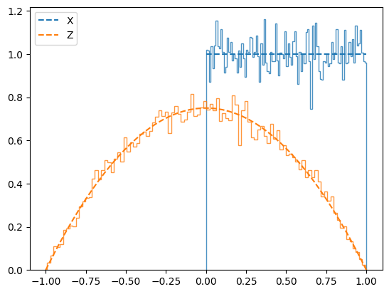
Let \(z=f(x)\) be some function. The variable \(Z=f(X)\) has PDF

\[\begin{align*} P_Z(z) &= \int \delta\Bigl(z - f(x)\Bigr) P_X(x)\d{x},\\ &= \int \delta\Bigl(z - f\Bigr) P_X(x) \overbrace{\left\lvert\diff{x}{f}\right\rvert}^{\abs{1/f'(x)}}\d{f}, \qquad f = f(x), \\ &= \sum_{x | f(x)=z}\frac{P_X(x)}{\abs{f'(x)}}, \end{align*}\]

where the sum is over all independent solutions to \(f(x) = z\).

Example: Generating a Random Distributions

Suppose you want to generate samples for a variable \(Z\) with PDF \(P_Z(z)\). You can use this result to transform a variable generated with PDF \(P_X(x)\) by choosing \(Z = f(X)\) for an appropriate monotonic function \(f(x)\) which satisfies:

\[\begin{gather*} f'(x) = \frac{P_X(x)}{P_Z(f(x))}, \qquad P_Z(f)\d{f} = P_X(x)\d{x}, \\ C_Z\Bigl(f(x)\Bigr) = \int_{-\infty}^{f(x)} P_Z(z) \d z = \int_{-\infty}^{x} P_X(x)\d{x} = C_X(x),\\ f(x) = C_Z^{-1}\Bigl(C_X(x)\Bigr). \end{gather*}\]

Here \(C_X(x)\) and \(C_Z(z)\) are the cumulative distribution functions (CDFs) for \(X\) and \(Z\) respectively. For example, suppose you want to generate a set if points \(z \in [-1, 1]\) with distribution \(P_Z(z) = 3(1-z^2)/4\) from a variable \(x \in [0, 1]\) with uniform distribution \(P_X(x) = 1\). We have:

\[\begin{gather*} C_Z(z) = \int_{-1}^z\d{z} P_Z(z) = \frac{-z^3 + 3z + 2}{4}, \\ C_X(x) = \int_{0}^{x}\d{x} P_X(x) = x,\\ z = f(x) = C_Z^{-1}(C_X(x)) = C_Z^{-1}(x). \end{gather*}\]

This involves finding the roots of a cubic polynomial, but this is easily done numerically with a few steps of Newtons’s method starting with a good guess. (See global_newton for details.)

def C_Z_inv(x):
    """Return z where x = C_Z(z)."""
    z = 2/np.pi * np.arcsin(2*x-1) # Good initial guess
    for _n in range(4):            # 4 steps give machine precision
        z -= ((np.polyval([-1, 0, 3, 2], z) - 4*x) 
              / (np.polyval([-3, 0, 3], z) + 1e-32))
    return z

rng = np.random.default_rng(seed=2)
X = rng.random(size=20000)  # Uniform distribution of X from 0 to 1
Z = C_Z_inv(X)

x = np.linspace(0, 1)
z = np.linspace(-1, 1)


fig, ax = plt.subplots()
kw = dict(histtype='step', alpha=0.8, density=True)
plt.hist(X, bins=100, ec="C0", **kw)
plt.hist(Z, bins=100, ec="C1", **kw)
plt.plot(x, 0*x + 1, '--C0', label='X')
plt.plot(z, 3*(1-z**2)/4, '--C1', label='Z')
ax.legend();

Sum of Independent Random Variables

The distribution of the sum \(Z = X+Y\) of two independently distributed random variavles is thus the convolution \(P_{X+Y} = P_X * P_Y\) of the distributions:

\[\begin{gather*} P_{X+Y}(z) = \iint\d{x}\d{y}\;\delta(x + y - z)P_X(x)P_Y(y) = \int_{-\infty}^{\infty}\!\!\!\d{x}\;P_X(x)P_Y(z-x). \end{gather*}\]

Example: Sum of Independent Normal Distributions

The sum or normally distributed random variables over the same space is also normal with the following mean and covariance matrix

\[\begin{gather*} \vect{\mu}_Z = \vect{\mu}_X + \vect{\mu}_Y, \qquad \mat{C}_{Z} = \mat{C}_X + \mat{C}_Y. \end{gather*}\]

If the spaces are not the same, then the vectors and matrices must be organized appropriately so corresponding spaces overlap, with the other spaces add in separate dimensions.

Note: The distributions must be independent, or at least jointly normal, otherwise the resulting distribution might not be a multivariate normal distribution.

Product of Independent Random Variables

Here do the \(y\) integral by changing variables to \(f = f(y) = xy\) so that \(f\) appears directly in \(\delta\bigl(f(y) - z\bigr)\). The change of variables thus gives \(\d{y} = \d{f}/\abs{f'(y)} = \d{y}/\abs{x}\).

The distribution of the product \(Z = XY\) of two independently distributed random variables is:

\[\begin{gather*} P_{XY}(z) = \iint\d{x}\d{y}\;\delta(xy - z)P_X(x)P_Y(y) = \int_{-\infty}^{\infty}\!\!\!\d{x}\frac{P_X(x)P_Y(z/x)}{\abs{x}}. \end{gather*}\]

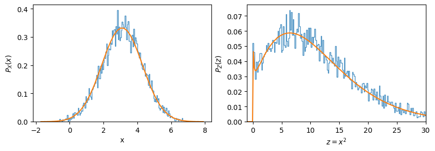
Example: Square of a Normal Variable

Let \(X\) be normally distributed, then \(Z = X^2\) has the following distribution:

\[\begin{gather*} P_Z(z) = \sum_{x = \pm \sqrt{z}} \frac{P_X(x)}{2\abs{x}} = \Theta(z) \frac{e^{-(\sqrt{z}-\mu)^2/2\sigma^2} + e^{-(-\sqrt{z}-\mu)^2/2\sigma^2}} {2\sqrt{2\pi z \sigma^2}}. \end{gather*}\]

If the mean is zero, then this simplifies:

\[\begin{gather*} P_Z(z) = \Theta(z) \frac{e^{-z/2\sigma^2}}{\sqrt{2\pi z \sigma^2}}. \end{gather*}\]

If the spaces are not the same, then the vectors and matrices must be organized appropriately so corresponding spaces overlap, with the other spaces add in separate dimensions.

Note: The distributions must be independent, or at least jointly normal, otherwise the resulting distribution might not be a multivariate normal distribution.

Working with random variables is fraught with opportunities to make algebraic mistakes, forgetting factors of 2 etc. Checking with code is almost trivial, so do it! (The hardest part is choosing good parameters for the histograms.)

rng = np.random.default_rng(seed=2)

mu = 3.1
sigma = 1.2

N = 10000
X = rng.normal(loc=mu, scale=sigma, size=N)
Z = X**2
x = np.linspace(mu-4*sigma, mu+4*sigma)
z = np.linspace(-1, 30, 200)

def P_X(x):
    return (np.exp(-(x-mu)**2/2/sigma**2)
            / np.sqrt(2*np.pi * sigma**2))

def P_Z(z):
    x = np.sqrt(abs(z))
    df_dx = 2*abs(x)
    return np.where(z < 0, 0, (P_X(x) + P_X(-x))/df_dx)

kw = dict(histtype='step', alpha=0.8, density=True)
fig, axs = plt.subplots(1, 2, figsize=(10, 3))
ax = axs[0]
ax.hist(X, 200, **kw)
ax.plot(x, P_X(x))
ax.set(xlabel="x", ylabel="$P_X(x)$")

ax = axs[1]
ax.hist(Z, bins=z, **kw)
ax.plot(z, P_Z(z), '-', scaley=False)
ax.set(xlim=(-1, 30), xlabel="$z=x^2$", ylabel="$P_Z(z)$");

Chi-Squared Distribution

As an extended example, consider the \(\chi^2\) distribution for a linear model with normally distributed errors \(e_n\), each with mean \(0\) and variance \(\sigma_n^2\). Then, we have:

\[\begin{gather*} \chi^2 = \sum_n \left(\frac{f(x_n, \vect{a}) - y_n}{\sigma_n}\right)^2 = \sum_n \frac{e_n^2}{\sigma_n^2} = \sum_n \tilde{e}_n^2. \end{gather*}\]

Let \(\tilde{e}_n = e_n/\sigma_n\). We have the following PDFs:

\[\begin{align*} P_{e_n}(x) &= \frac{e^{-x^2/2/\sigma_n^2}}{\sqrt{2\pi \sigma_n^2}}\\ P_{\tilde{e}_n}(x) &= \frac{P_{e_n}(\sigma_n x)}{\d{\tilde{e}_n}/\d{e_n}} = \sigma_n P_{e_n}(\sigma_n x) = \frac{e^{-x^2/2}}{\sqrt{2\pi}}\\ P_{\tilde{e}_n^2}(x) &= \Theta(x) \frac{e^{-x/2}}{\sqrt{2\pi x}}\\ P_{\chi^2, \nu}(x) &= P_{\text{poisson}}(k;x/2) = \Theta(x) \frac{(x/2)^k e^{-x/2}}{k!} \qquad k = \frac{\nu}{2} - 1\\ &= \Theta(x)\frac{x^{\nu/2-1} e^{-x/2}}{2^{\nu/2-1}\Gamma(\nu/2)}. \end{align*}\]

The last step involves adding independent distributions, which is done with convolution and gives the chi-square distribution as described in section 6.14.8 of [Press et al., 2007]. This can be computed using scipy.stats.chi2. It has mean \(\nu\) and variance \(2\nu\). From this, we can also compute the distribution for \(\chi^2_r\):

\[\begin{align*} P_{\chi^2, \nu}(\chi^2) &= \Theta(\chi^2)\frac{(\chi^2)^{\nu/2-1} e^{-\chi^2/2}}{2^{\nu/2-1}\Gamma(\nu/2)}, & \mu &= \nu, & \sigma &= \sqrt{2\nu}\\ P_{\chi^2_r, \nu}(\chi^2_r) &= \nu P_{\nu}(\chi^2) = \nu P_{\chi^2, \nu}(\nu\chi^2_r), & \mu &= 1, & \sigma &= \sqrt{2/\nu}. \end{align*}\]

The proof is simple: first transform to variables \(\vect{x} = \mat{L}(\vect{a} - \bar{\vect{a}})\) by factoring \(\mat{C} = \mat{L}\mat{L}^T\), then note that \(\chi^2(\vect{a}) = \norm{\vect{x}}^2\) is just a sum of \(\nu\) independently distributed normal variables with zero mean and unit variance.

The chi-squared distribution also arises when determining confidence regions of a multivariate normal distribution of \(\nu\) parameters \(\vect{a}\) with mean \(\bar{\vect{a}}\) and covariance matrix \(\mat{C}\):

\[\begin{gather*} P(\vect{a}) = \frac{ \exp\Bigl( -\frac{1}{2} \overbrace{ (\vect{a} - \bar{\vect{a}})^T \cdot\mat{C}^{-1} \cdot(\vect{a} - \bar{\vect{a}}) }^{\chi^2(\vect{a})} \Bigr) }{ \sqrt{\det{(2\pi\mat{C})}} } = P_{\chi^2, \nu}\bigl(\chi^2(\vect{a})\bigr). \end{gather*}\]

from scipy.stats import chi2, norm

chi2_rs = np.linspace(-0.1, 4, 100)
fig, axs = plt.subplots(1, 2, figsize=(10, 3))
for nu in [1, 2, 3, 4, 20, 50, 100]:
    chi2s = chi2_rs * nu
    l0, = axs[0].plot(chi2s, chi2.pdf(chi2s, df=nu), label=rf"$\nu={nu}$")
    l1, = axs[1].plot(chi2_rs, nu*chi2.pdf(nu*chi2_rs, df=nu), label=rf"$\nu={nu}$")
    axs[0].plot(chi2s, np.exp(-(chi2s - nu)**2/4/nu)/np.sqrt(4*np.pi*nu),
                ':', c=l0.get_c())
    sigma = np.sqrt(2/nu)
    axs[1].plot(chi2_rs, np.exp(-(chi2_rs - 1)**2/2/sigma**2)/np.sqrt(2*np.pi*sigma**2),
                ':', c=l1.get_c())
    mean_chi2, var_chi2 = chi2.stats(df=nu, moments='mv')
    print(f"𝜈={nu}, χ² mean={mean_chi2}, var={var_chi2}")

axs[0].set(xlabel=r"$\chi^2$", ylabel=r"$P_{\chi^2, \nu}(\chi^2)$", 
           xlim=(-0.1, 20), ylim=(0, 0.6))
axs[1].set(xlabel=r"$\chi^2_r$", ylabel=r"$P_{\chi^2_r, \nu}(\chi^2_r)$")
for ax in axs:
    ax.legend();

𝜈=1, χ² mean=1.0, var=2.0
𝜈=2, χ² mean=2.0, var=4.0
𝜈=3, χ² mean=3.0, var=6.0
𝜈=4, χ² mean=4.0, var=8.0
𝜈=20, χ² mean=20.0, var=40.0
𝜈=50, χ² mean=50.0, var=100.0
𝜈=100, χ² mean=100.0, var=200.0

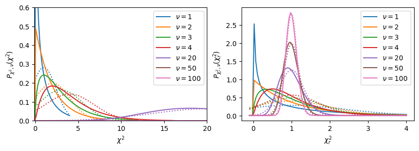
These results indicate why it is important to work out the confidence intervals carefully. If there are many degrees of freedom \(\nu > 20\), then \(\chi^2_r\) is tightly peaked with \(\sigma = \sqrt{2/\nu}\) about the mean value of \(1\) (dotted lines):

\[\begin{gather*} \lim_{\nu \rightarrow \infty} P_{\chi^2_r, \nu}(\chi^2_r) \rightarrow \frac{e^{-(\chi^2_r - 1)^2/(4/\nu)}}{\sqrt{4\pi/\nu}}. \end{gather*}\]

But, if you have limited data, then the distribution has some significant deviations and you should use the CDF of the actual \(\chi^2\) distribution to compute your confidence intervals.

Why \(\nu = N - M\)?

Try proving this yourself. The geometry discussed in geometry-of-fitting might help. The basic idea is that, for any realization, \(M\) of the errors can be eliminated by adjusting the parameters for the best fit, leaving \(\nu = N-M\) independent errors which must be combined to get \(P_{\chi^2, \nu}(\chi^2)\).

When performing an actual maximum likelihood analysis, the distribution of \(\chi^2\) after minimizing is a [chi-square distribution] with \(\nu = N-M\) where there are \(N\) data points and \(M\) parameters in the model. This comes from the fact that we don’t compute \(f(x_n, \vect{a})\) with \(\vect{a}\) being the physical parameters as assumed in the model \(y_n = f(x_n, \vect{a}) + e_n\), but rather, we compute \(f(x_n, \bar{\vect{a}})\) where \(\bar{\vect{a}}(\vect{e}) \neq \vect{a}\) maximizes the likelihood for a given set of data, and therefore, depends on \(\vect{e}\). This additional dependence reduces \(\nu\) from \(N\) to \(\nu = N-M\).

Confidence Regions

We use here what is sometimes called the “highest density confidence region” or HDR, which is one of the possible credible regions. Other options include central regions, or equal-tailed intervals (in 1D). For a gaussian these are the same, but differ for multi-modal distributions especially where the HDR will be disjoint.

Another reason that the chi square distribution is useful is to find confidence regions. Give a set of \(\nu\) random variables distributed as \(P(\vect{a})\). The HDR confidence region with confidence level \(p\) is the region where \(P(\vect{a}) < P_{p}\) such that \(100p\%\) of the results like within this region (i.e. \(p=0.95\) corresponds to a \(95\%\) confidence level):

\[\begin{gather*} \int_{\mathrlap{P(\vect{a}) < P_p}}\d^{\nu}\vect{a}\; P(\vect{a}) = p. \end{gather*}\]

If \(P(\vect{a})\) is a multivariate normal distribution with zero norm, then we can transform to \(\chi^2\) which is distributed as above, solving the problem:

\[\begin{gather*} \int_{\mathrlap{P(\vect{a}) < P_p}}\d^{\nu}\vect{a}\; P(\vect{a}) = \int_0^{\chi^2_p}\d{\chi^2}P_{\chi^2, \nu}(\chi^2) = p(\chi^2_p). \end{gather*}\]

Hence, \(p(\chi^2_p)\) is just the CDF of the chi square distribution with \(\nu\) degrees of freedom, and the appropriate value of \(\chi^2_p\) is the inverse of this, which can be computed using the scipy.stats.rv_continuous.ppf() method of the scipy.stats.chi2 distribution:

Here we get the \(n\sigma\) confidence levels from a gaussian distribution:

\[\begin{gather*} p = \int_{-n}^{n}\d{x}\;\frac{e^{-x^2/2}}{\sqrt{2\pi}}. \end{gather*}\]

from scipy.stats import chi2, norm

sigmas = [1, 2, 3, 4]
ps = norm.cdf(np.sqrt(sigmas)) - norm.cdf(-np.sqrt(sigmas))
print("Confidence levels:")
print(", ".join([f"{100*_p:.2f}% ({_n}σ)" for _n, _p in zip(sigmas, ps)]))
for nu in [1, 2, 3, 4]:
    print(f"χ²ₚ (𝜈={nu}): {chi2.ppf(ps, df=nu).round(2)}")

Confidence levels:
68.27% (1σ), 84.27% (2σ), 91.67% (3σ), 95.45% (4σ)
χ²ₚ (𝜈=1): [1. 2. 3. 4.]
χ²ₚ (𝜈=2): [2.3  3.7  4.97 6.18]
χ²ₚ (𝜈=3): [3.53 5.21 6.67 8.02]
χ²ₚ (𝜈=4): [4.72 6.62 8.24 9.72]

Note that for \(\nu = 1\) degree of freedom, the \(n\sigma\) confidence regions correspond to \(\chi^2_p = n\), but for higher dimensions, this is not the case.

To see that the distribution is equivalent to the chi squared distribution, note that

\[\begin{gather*} P(\vect{a}) = \frac{ \exp\Bigl( -\frac{1}{2}\overbrace{\vect{a}^T\mat{C}^{-1}\vect{a}}^{\chi^2} \Bigr)}{\sqrt{\det(2\pi \mat{C})}} = \frac{ \exp\Bigl( -\frac{1}{2}\vect{x}^T\vect{x} \Bigr)}{\sqrt{\det(2\pi \mat{C})}} = \frac{ \exp\Bigl(-\frac{\chi^2(\vect{a})}{2}\Bigr)}{\sqrt{\det(2\pi \mat{C})}}. \end{gather*}\]

Obtain \(\mat{L}\) using either a Cholesky decomposition or by diagonalizing \(\mat{C} = \mat{U}\mat{D}\mat{U}^T\), \(\mat{L} = \mat{U}\sqrt{\mat{D}}\).

where we first transform to a new set of variables \(\vect{x}\) such that \(\vect{a} = \mat{L}\vect{x}\) where \(\mat{C} = \mat{L}\mat{L}^T\). Here each components of \(\vect{x}\) is independently distributed with a zero-mean, \(\sigma=1\) normal distribution. We then transform to \(\chi^2\) which is the sum of \(\nu\) squares of such distributions, giving \(P_{\chi^2, \nu}(\chi^2)\) as computed above.

The normalization factor changes with a determinant of the Jacobian \(\det\mat{L} = \sqrt{\det\mat{C}}\) so we have:

\[\begin{gather*} P(\vect{x}) = \sqrt{\det\mat{C}} P(\vect{a}) = \frac{1}{\sqrt{(2\pi)^\nu}} \exp\Bigl( -\frac{1}{2}\vect{x}^T\vect{x} \Bigr). \end{gather*}\]