12. Asymptotic Series

12. Asymptotic Series#

Gaussian Perturbation#

In Zee’s book [Zee, 2010], he considers the following “baby problem” of computing the integral

\[\begin{gather*} Z(J) = \int_{-\infty}^{\infty}\d{q}\;e^{-\frac{1}{2}m^2q^2 - \frac{\lambda}{4!}q^4 + Jq}. \end{gather*}\]

He uses this as an example for explaining Feynman rules with a close connection to scalar field theory. For our purposes we will simplify this by setting \(m=1\) and calling \(\epsilon = \lambda /4!\). Through some tricks, he notes that this can be expressed as

\[\begin{gather*} Z(J,\epsilon) = \int_{-\infty}^{\infty}\d{q}\;e^{-\frac{1}{2}q^2 - \epsilon q^4 + Jq} = \sqrt{2\pi}\exp\left(-\epsilon\diff[4]{}{J}\right) \exp\left(\frac{J^2}{2}\right) \end{gather*}\]

suggesting that the solution might be expressed as a power series in \(\epsilon\):

\[\begin{align*} \frac{Z(J,\epsilon)}{\sqrt{2\pi}} &= \Biggl( 1 - \epsilon\diff[4]{}{J} + \frac{\epsilon^2}{2!}\diff[8]{}{J} - \frac{\epsilon^3}{3!}\diff[12]{}{J} + O(\epsilon^4) \Biggr)e^{J^2/2}\\ & \begin{multlined} = e^{J^2/2}\Biggl(1 - \epsilon(J^4 + 6J^2 + 3)\\ + \frac{\epsilon^{2}}{2!}(J^{8} + 28 J^{6} + 210 J^{4} + 420 J^{2} + 105) \\ - \frac{\epsilon^{3}}{3!}(J^{12} + 66 J^{10} + 1485 J^{8} + 13860 J^{6} + 51975 J^{4} + 62370 J^{2} + 10395)\\ + O(\epsilon^4)\Biggr). \end{multlined} \end{align*}\]

For example, we can express \(Z(0, \epsilon)\) as

\[\begin{gather*} \frac{Z(0, \epsilon)}{\sqrt{2\pi}} = \sum_{n=0}^{\infty} a_n \epsilon^n = \sum_{n=0}^{\infty} \frac{(4n-1)!!}{n!} (-\epsilon)^{n} = 1 - 3\epsilon + \frac{105}{2} \epsilon^{2} + O(\epsilon^{3}). \end{gather*}\]

and expand \(Z(J, \epsilon)\) as (second order term not checked yet)

\[\begin{gather*} \frac{Z(J,\epsilon)}{Z(J,0)} = \sum_{n=0}^{\infty} \frac{(4n-1)!!}{n!} (-\epsilon)^{n} + J^2\sum_{n=1}^{\infty} \frac{(4n-1)!! (2n)}{n!} (-\epsilon)^{n} + O(J^4). \end{gather*}\]

The question we want to ask here is: how well do such series converge? Such series are called asymptotic series in the sense that, for a fixed number of terms \(N\), they converge for small \(\epsilon\). To be precise

(Asymptoticity)

A power series \(\sum_{n=0}^{\infty} a_n \epsilon^n\) is said to be asymptotic to a function \(f(\epsilon)\) if, for fixed \(N\) and sufficiently small \(\epsilon\):

\[\begin{gather*} \left| f(\epsilon) - \sum_{n=0}^{N} a_n \epsilon^n\right| \sim O(\epsilon^{N+1}). \end{gather*}\]

(See [Boyd, 1999] for details.)

Note that this is not what we typically want in terms of convergence. Rather, we would like to know that, for sufficiently small but fixed \(\epsilon\), the power series will converge as the number \(N\) of terms included increases. This switches the order of these, fixing \(N\) instead and requiring sufficiently fast converges for small \(\epsilon\).

[Boyd, 1999] contains a lot of wisdom about such asymptotic series, including heuristics about when an expansion might be asymptotic. One heuristic is that the asymptotic series will be best if truncated at \(n = N\) once the terms stop decreasing.

Here we demonstrate some properties of the asymptoticity of the expansion for \(F(\epsilon) = Z(0, \epsilon)/\sqrt{2\pi}\).

from functools import partial
from scipy.special import factorial, factorial2
from scipy.integrate import quad

def f(q, eps):
    return np.exp(-q**2/2-eps*q**4)/np.sqrt(2*np.pi)

def F(eps):
    return quad(partial(f, eps=eps), -np.inf, np.inf, epsabs=1e-13, epsrel=1e-13)[0]

epss = np.linspace(0, 0.1, 1000)
fig, ax = plt.subplots()
ns = np.arange(50)
ax.plot(epss, list(map(F, epss)), ':k')
ylim = ax.get_ylim()

def coeff(n):
    if n < 1:
        return 1
    return factorial2(4*n-1)/factorial(n)

for N in range(1, 10):
    ax.plot(epss, np.sum([coeff(n)*(-epss)**n for n in range(N)], axis=0), 
    '-', label=f"{N=}")
ax.legend()
ax.set(xlabel="$\epsilon$", ylabel="$F(\epsilon)$", ylim=ylim);

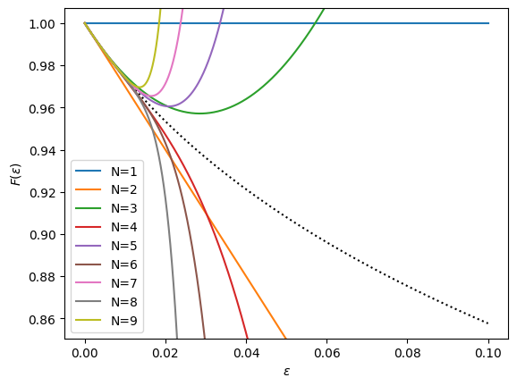
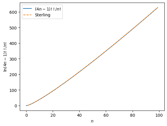
_images/9d1199b70b8f04c2054e6eb93d4c6173f73d4b1e08e35aed21ce9e0397e9d6ef.png

Here we start to see the problem: higher order approximations better match the behaviour of \(F(\epsilon)\) for small \(\epsilon\), but diverge more and more quickly. This suggests that the radius of convergence is small, and indeed, it is zero here. Considering the series, this is reasonable since the coefficients \((4n-1)!!/n! \sim n^{n-1/2}\) (using Sterling’s approximation) will always eventually dominate over the powers of \(\epsilon^n\):

\[\begin{gather*} \abs{a_n} = \frac{(4n-1)!!}{n!} \sim \frac{(16n\epsilon/e)^{n}}{\sqrt{\pi n}}. \end{gather*}\]

For a given \(\epsilon\), the terms have a minimum magnitude for \(n=N\) when

\[\begin{gather*} \epsilon \approx \frac{e^{1/2N}}{16 N}, \qquad a_{N}\epsilon^{N} \sim \sqrt{\frac{e}{\pi N}}e^{-N}. \end{gather*}\]

Since the series is alternating, a good approximation for the error obtained by truncating at \(n=N\):

\[\begin{gather*} N \approx \frac{1}{2\ln(16 \epsilon N)}, \qquad E(N) \sim \sqrt{\frac{e}{\pi N}}e^{-N} \approx 4\sqrt{\frac{e\epsilon}{\pi}}e^{-1/16\epsilon}. \end{gather*}\]

As we shall see below, this is actually a pretty good approximation. With this optimal truncation, the approximation is what is called superasymptotic (see [Boyd, 1999]). Superasymptotic approximations typically have an optimal truncation \(N \propto 1/\epsilon\) with an error \(O\bigl(\exp(-c/\epsilon)\bigr)\). In our

(Superasymptotic)

An optimally-truncated asymptotic series is a superasymptotic approximation. Typically power series \(\sum_{n=0}^{\infty} a_n \epsilon^n\) is said to be asymptotic to a function \(f(\epsilon)\) if, for fixed \(N\) and sufficiently small \(\epsilon\):

\[\begin{gather*} \left| f(\epsilon) - \sum_{n=0}^{N} a_n \epsilon^n\right| \sim O(\epsilon^{N+1}). \end{gather*}\]

(See [Boyd, 1999] for details.)

Details

To estimate when the terms will stop decreasing, we can use Sterling’s approximation

\[\begin{gather*} \lim_{n\rightarrow\infty} \frac{n!}{(n/e)^n \sqrt{2\pi n}} = 1 \end{gather*}\]

applied to

\[\begin{gather*} (2n)!! = 2^n n! \sim \sqrt{2\pi n} (2n/e)^{n}, \\ (2n-1)!! = \frac{(2n)!}{(2n)!!} \sim %\frac{\sqrt{4\pi n} (2n/e)^{2n}}{\sqrt{2\pi n} (2n/e)^{n}} = \sqrt{2} (2n/e)^{n},\\ (4n-1)!! \sim \sqrt{2} (4n/e)^{2n},\\ \frac{(4n-1)!!}{n!} \sim \frac{(16n/e)^{n}}{\sqrt{\pi n}}. \end{gather*}\]

The terms have a minimum size \(n=N\) when

\[\begin{gather*} 0 \approx \left.\diff{}{n}\frac{(4n-1)!!}{n!}\epsilon^n\right|_{n=N} \sim \diff{}{n} \frac{(16n\epsilon/e)^{n}}{\sqrt{\pi n}} \propto n\log(16\epsilon n) - \frac{1}{2},\\ \epsilon \approx \frac{e^{1/2N}}{16 N}, \qquad a_N\epsilon^{N} \sim \sqrt{\frac{e}{\pi N}}e^{-N} \end{gather*}\]

Since this is an alternating series, the size of the omitted term provides an estimate of the error. (Technically, we should hold \(\epsilon\) fixed, but use \(n=N+1\). This gives:)

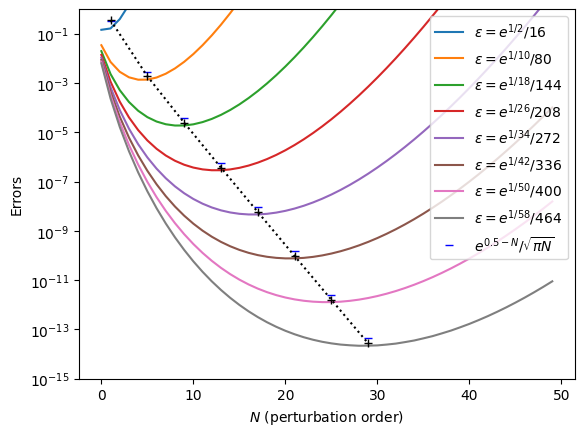
\[\begin{gather*} E(N) \sim \frac{(1+N^{-1})^{N+1} \sqrt{e}^{N^{-1} - 1}}{\sqrt{\pi (N+1)}}e^{-N} \approx (1+N^{-1})^{N+1} e^{1/2N} \sqrt{\frac{e}{\pi (N+1)}}e^{-(N+1)} \end{gather*}\]

_images/7df6223481d8da17ea47be1feb7b5bfc3da00bf947566c6af825ef1dedeb62a4.png

The black pluses above represent our error estimate \(E(N)\) after optimally truncating at the \(n=N\) which minimizes the size of the terms \(a_n\epsilon^n\) and the blue lines represent the simplified upper bound of the \(N\)’th term given above.

import sympy
m, J, eps = sympy.var(r'm,J,\epsilon')
m = 1
f = sympy.exp(J**2/2/m**2)
c = 1
terms = []
N = 10
for n in range(N):
    terms.append(c*f.subs(dict(J=0)).simplify())
    f = f.diff(J, J, J, J).simplify()
    c *= eps
[t.subs([(eps, 1)]) for t in terms]

[1,
 3,
 105,
 10395,
 2027025,
 654729075,
 316234143225,
 213458046676875,
 191898783962510625,
 221643095476699771875]

Analytic Solution#

We note that \(Z(0, \epsilon)\) has an analytic solution:

\[\begin{gather*} Z(0, \epsilon) = \int_{-\infty}^{\infty}\d{q}\; e^{-q^2/2 - \epsilon q^4} = \frac{2\sqrt[32\epsilon]{e}K_{1/4}(1/32\epsilon)}{\sqrt{32\epsilon}}, \end{gather*}\]

where \(K_{\alpha}(x)\) is the modified Bessel function of the second kind, which satisfies:

\[\begin{gather*} x^2 \diff[2]{y}{x^2} + x\diff{y}{x} - (x^2 + \alpha^2)y = 0,\\ K_{\alpha}(x) = \int_0^{\infty}\d{t}\; e^{-x\cosh t}\cosh \alpha t = \int_0^{\infty}\d{t}\; e^{-x\cosh t}\cosh \alpha t. \end{gather*}\]

Cumulants#

Consider the following power series:

\[\begin{gather*} 1 + \sum_{n=1}^{\infty} m_n\frac{t^n}{n!} = \exp\left( \sum_{n=1}^{\infty} \kappa_n \frac{t^n}{n!}. \right) \end{gather*}\]

Ignoring issues of convergence, one can algebraically express the coefficients \(m_n\) (called the moments) in terms of the coefficients \(\kappa_n\) (called the cumulants). This is the subject of formal cumulants.

Log of a Series#

Suppose that

\[\begin{gather*} Z(x) = 1 - \sum_{m=1}^{\infty} c_m x^m\\ \ln(1-x) = -\sum_{n=1}^{\infty} \frac{x^n}{n},\\ \ln Z(x) = -\sum_{n=1}^{\infty} \frac{[1-Z(x)]^n}{n} = -\sum_{n=1}^{\infty} \frac{\Bigl(\sum_{m=1}^{\infty} c_m x^m\Bigr)^n}{n},\\ \end{gather*}\]

Borel Resummation#

How do we work with such asymptotic series? Well, if our coupling constant happens to be small enough, then we can take advantage of the superasymptotic approximation to get extremely high precision with relatively little work computing to order \(N\sim 1/\epsilon\) and stopping. This is what is typically done in the Standard Model, especially in QED where the small parameter is the fine-structure constant \(\alpha = 1/137.035999084(21)\). Asymptoticity of QED means that we can keep improving to roughly order 137 in perturbation theory, and is the reason QED is one of the most spectacularly accurate scientific theories.

On the other hand, asymptoticity also means that we can’t keep gaining precision - at some point the series will start diverging. Through arguments along these lines, it is known that the Standard Model as currently formulated cannot be the final theory of everything (ToE).

Suppose we are faced with an asymptotic series, but we need better control. How can we proceed? Many strategies are discussed in [Bender and Orszag, 1999], but a common technique is to use Borel resummation. The idea is simple, given a power series

\[\begin{gather*} F(\epsilon) = \sum_{n=0}^{\infty}f_n\epsilon^{n}, \end{gather*}\]

we define the Borel transform as

\[\begin{gather*} \mathcal{B}F(\epsilon) = \sum_{n=0}^{\infty}\frac{f_n}{n!}\epsilon^{n} \end{gather*}\]

The additional factor here of \(n!\) in the denominator should assure that \(\mathcal{B}F(\epsilon)\) converges in many cases where \(F(\epsilon)\) does not. If the Borel transformation converges for all positive real numbers, then we can define the Borel sum of \(F\) as

\[\begin{gather*} \int_0^{\infty}\d{t}\;e^{-t}\mathcal{B}F(t\epsilon). \end{gather*}\]

A weaker form is to extend the partial sums:

\[\begin{gather*} \lim_{t\rightarrow \infty} e^{-t}\sum_{n=0}^{\infty} \frac{t^n}{n!}F_n(\epsilon), \qquad F_n(\epsilon) = \sum_{n=0}^{N}f_n \epsilon^n. \end{gather*}\]

import sympy
q, eps = sympy.var('q,\epsilon', positive=True)
Q = 2*sympy.exp(-q**2/2-eps*q**4).integrate((q, 0, sympy.oo))
Q = 2*sympy.exp(-eps*q**4).integrate((q, 0, sympy.oo))
Q

\[\displaystyle \frac{\Gamma\left(\frac{1}{4}\right)}{2 \sqrt[4]{\epsilon}}\]

Assessment#

The following are divergent asymptotic series in the parameter \(\epsilon\). Explain (heuristically) why.

Stieltjes Function#

\[\begin{gather*} S(\epsilon) = \int_0^{\infty}\d{t}\; \frac{e^{-t}}{1+\epsilon t} \end{gather*}\]

Zee’s Baby Problem#

\[\begin{gather*} Z(\epsilon) = \int_{-\infty}^{\infty}\d{q}\; e^{-q^2/2 - \epsilon q^4}. \end{gather*}\]

Anharmonic Oscillator#

The ground state energy \(E(\epsilon)\) of the following anharmonic oscillator potential in quantum mechanics:

\[\begin{gather*} V(x) = \frac{m\omega^2}{2}x^2 + \epsilon x^4. \end{gather*}\]

Linear Differential Equations#

\[\begin{gather*} \epsilon^2 u''(x) - u(x) = -f(x) \end{gather*}\]

where both \(\abs{f(x)} \rightarrow 0\) and \(\abs{u(x)} \rightarrow 0\) as \(\abs{x} \rightarrow \infty\).