Show code cell content

Hide code cell content

import mmf_setup;mmf_setup.nbinit()
import logging;logging.getLogger('matplotlib').setLevel(logging.CRITICAL)
%matplotlib inline
import numpy as np, matplotlib.pyplot as plt

$\newcommand{\vect}[1]{\mathbf{#1}} \newcommand{\uvect}[1]{\hat{#1}} \newcommand{\abs}[1]{\lvert#1\rvert} \newcommand{\norm}[1]{\lVert#1\rVert} \newcommand{\I}{\mathrm{i}} \newcommand{\ket}[1]{\left|#1\right\rangle} \newcommand{\bra}[1]{\left\langle#1\right|} \newcommand{\braket}[1]{\langle#1\rangle} \newcommand{\Braket}[1]{\left\langle#1\right\rangle} \newcommand{\op}[1]{\mathbf{#1}} \newcommand{\mat}[1]{\mathbf{#1}} \newcommand{\d}{\mathrm{d}} \newcommand{\D}[1]{\mathcal{D}[#1]\;} \newcommand{\pdiff}[3][]{\frac{\partial^{#1} #2}{\partial {#3}^{#1}}} \newcommand{\diff}[3][]{\frac{\d^{#1} #2}{\d {#3}^{#1}}} \newcommand{\ddiff}[3][]{\frac{\delta^{#1} #2}{\delta {#3}^{#1}}} \newcommand{\floor}[1]{\left\lfloor#1\right\rfloor} \newcommand{\ceil}[1]{\left\lceil#1\right\rceil} % The following allows KaTeX to render these for significantly improved % performance on CoCalc. \newcommand{\DeclareMathOperator}[2]{\newcommand{#1}{#2}} \DeclareMathOperator{\Tr}{Tr} \DeclareMathOperator{\erf}{erf} \DeclareMathOperator{\erfi}{erfi} \DeclareMathOperator{\sech}{sech} \DeclareMathOperator{\sn}{sn} \DeclareMathOperator{\cn}{cn} \DeclareMathOperator{\dn}{dn} \DeclareMathOperator{\sgn}{sgn} \DeclareMathOperator{\order}{O} \DeclareMathOperator{\diag}{diag} % \newcommand{\mylabel}[1]{\label{#1}\tag{#1}} \newcommand{\degree}{\circ}$

This cell adds /home/docs/checkouts/readthedocs.org/user_builds/physics-571-math-methods/checkouts/latest/src to your path, and contains some definitions for equations and some CSS for styling the notebook. If things look a bit strange, please try the following:

• Choose "Trust Notebook" from the "File" menu.
• Re-execute this cell.
• Reload the notebook.

Deuteron

Heuristically, the nuclear interaction can be described by the exchange of pions, which gives an energy scale of \(m_\pi c^2 \approx 135\;\rm{MeV}\) and a length-scale of \(\hbar c/m_{\pi} \approx 0.56\;\rm{fm}\). Whereas exchange of massless particles like the photon give rise to a Coulomb-like potential \(V(r) \propto 1/r\), the exchange of massive particles yields a Yukawa potential:

\[\begin{gather*} V_{m}(r) = -g^2 \frac{e^{-\alpha m_{\pi} r /\hbar c}}{r}. \end{gather*}\]

Show code cell source

Hide code cell source

r = np.linspace(0.1, 3)
V = -np.exp(-r)/r
fig, ax = plt.subplots(figsize=(4,3))
ax.plot(r, V, label="Yukawa")
ax.plot(r, -1/r, label="Coulomb")
ax.legend()
ax.set(xlabel=r"$r$ [$\hbar c /\alpha m_{\pi}$]",
       ylabel=r"$V(r)/g^2$");

Here we say a little more about Example 8.3.3 in [Arfken et al., 2013]. The key physical idea is that the nuclear potential is short-ranged. Technically this means that it falls off faster than the Coulomb potential \(V \sim 1/r\), but

Specifically, we show that in the short-range limit, the potential has a peculiar structure. The naïve choice of \(V_0\delta^3(\vect{r})\) is too singular, but we need a combination of two parameters to get the correct short range boundary condition.

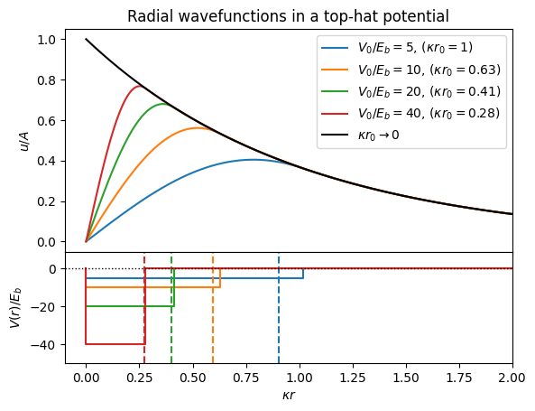
Example: Top-Hat Potential

To see this, consider an explicit realization of a top-hap potential \(V(r) = -V_0\Theta(r_0-r)\) with depth \(-V_0\) and range \(r_0\). The bound-states \(E = -E_b\) of the radial wavefunction have the following solutions

Here we use

\[\begin{gather*} \frac{\hbar^2k^2}{2m} - V_0 = \frac{-\hbar^2 \kappa^2}{2m} = -E_b, \end{gather*}\]

and the fact that both \(u(r)\) and \(u'(r)\) must be continuous at \(r_0\). We also note that \(kr_0 > \pi/2\) so let \(kr_0 = \tfrac{\pi}{2} + \alpha\) and use \(\cot(\tfrac{1}{2}\pi + \alpha) = -\tan(\alpha)\).

\[\begin{gather*} u(r) = \begin{cases} B\sin(k r) & r < r_0,\\ Ae^{-\kappa r} & r>r_0, \end{cases} \qquad \hbar \kappa = \sqrt{2mE_b}, \qquad \hbar k = \sqrt{2m(V_0 - E_b)},\\ B\sin(kr_0) = Ae^{-\kappa r_0}, \qquad kB\cos(kr_0) = -\kappa Ae^{-\kappa r_0}. \end{gather*}\]

Combining these, we have the transcendental equation.

\[\begin{gather*} \hbar k\cot(kr_0) = -\hbar k\tan(k r_0 - \tfrac{\pi}{2}) = -\hbar \kappa = -\sqrt{2mE_b},\\ kr_0 = \frac{\pi}{2} + \cot^{-1}\sqrt{\frac{V_0}{E_b}-1}. \end{gather*}\]

Taking \(V_0 \rightarrow \infty\), we can expand this to obtain the limiting behaviour in the short-range limit for fixed binding energy \(E_b\):

\[\begin{gather*} kr_0 = \frac{\pi}{2} + \sqrt{\frac{E_b}{V_0}} + \frac{1}{6}\sqrt{\frac{E_b}{V_0}}^3 + O(E_b/V_0)^5/2,\\ r_0 \rightarrow \frac{\pi}{2k} \approx \frac{\pi \hbar}{\sqrt{8mV_0}}\left( 1 + \frac{2}{\pi}\sqrt{\frac{E_b}{V_0}} + O\left(\frac{E_b}{V_0}\right) \right)\\ V_0 \rightarrow \frac{m\hbar^2}{2 r_0^2} \left( \pi^2 + 8\kappa r_0 + O(\kappa r_0)^2 \right). \end{gather*}\]

Details

Let \(x = E_b/V_0 \rightarrow 0\).

\[\begin{gather*} \cot^{-1} \sqrt{1/x - 1} = \sqrt{x} + \frac{x^{3/2}}{6} + O(x^{5/2})\\ \frac{1}{\sqrt{1-x}} = 1 + \frac{x}{2} + O(x^2)\\ \frac{\sqrt{2mV_0}}{\hbar}r_0 = \frac{\frac{\pi}{2} + \cot^{-1}\sqrt{1/x - 1}}{\sqrt{1-x}}\\ = \frac{\pi}{2} + \sqrt{x} + \frac{\pi}{4}x + \frac{2}{3}x^{3/2} + O(x^2)\\ = \frac{\pi}{2}\left(1 + \frac{2}{\pi}\sqrt{x} + \frac{1}{2}x + \frac{4}{3\pi}x^{3/2} + O(x^2)\right),\\ \frac{2}{\pi}\kappa r_0 = y = \sqrt{x} + \frac{2}{\pi}\sqrt{x}^2 + \frac{1}{2}\sqrt{x}^{3} + \frac{4}{3\pi}\sqrt{x}^{4} + O(\sqrt{x}^{5}),\\ \end{gather*}\]

We can then use the series reversion formula to compute

\[\begin{gather*} y = \sqrt{x} + a_2 \sqrt{x}^2 + a_3 \sqrt{x}^3 + \dots\\ \sqrt{x} = y + A_2y^2 + A_3y^3 + \cdots\\ \sqrt{x} = y - a_2y^2 + (2a_2^2 - a_3)y^3 + \dots = y - \frac{2}{\pi}y^2 + \left(\frac{8}{\pi^2} - \frac{1}{2}\right)y^3 + \dots. \end{gather*}\]

Then we have

\[\begin{gather*} V_0 = \frac{E_b}{x} = \frac{E_b}{(y+A_2y^2 + A_3y^3)^2} = \frac{E_b}{y^2(1+A_2y + A_3y^2)^2}\\ = \frac{E_b}{y^2}\left(1 - 2 A_2 y + (3A_2 - 2A_3)y^2 + (6A_2A_3 - 4A_2^3)y^3 + \cdots\right)\\ = \frac{E_b}{y^2}\left( 1 + \frac{4}{\pi} y + (1 - \tfrac{6}{\pi} - \tfrac{16}{\pi^2})y^2 + (\tfrac{6}{\pi} - \tfrac{64}{\pi^3})y^3 + \cdots\right)\\ = \frac{m\hbar^2 \kappa^2 \pi^2}{2\kappa^2 r_0^2} \left( 1 + \frac{8}{\pi^2}\kappa r_0 + (1 - \tfrac{6}{\pi} - \tfrac{16}{\pi^2})\tfrac{4}{\pi^2}(\kappa r_0)^2 + (\tfrac{6}{\pi} - \tfrac{64}{\pi^3})\tfrac{8}{\pi^3}(\kappa r_0)^3 + \cdots\right). \end{gather*}\]

Note: There is something wrong here with the higher order terms. Leading order works out.

The point of Shina Tan’s work [Tan, 2005] is introduce generalized delta-like “selectors” \(\lambda(\vect{r})\) and \(l(\vect{r})\) that are zero everywhere except \(\vect{r}=0\) and satisfy

\[\begin{gather*} \int \d^3{\vect{r}} \Bigl(a\lambda(\vect{r}) + b l(\vect{r})\Bigr) = a,\\ \int \d^3{\vect{r}} \Bigl(a\tfrac{\lambda(\vect{r})}{4\pi r} + b\tfrac{l(\vect{r})}{4\pi r}\Bigr) = b,\\ \int \d^3{\vect{r}} \Bigl(a\uvect{r}\lambda(\vect{r}) + b \uvect{r}l(\vect{r})\Bigr) = 0. \end{gather*}\]

These can be used to rigorously construct appropriate pseudo-potentials.

Note that this is a very peculiar limiting behaviour. The leading order behaviour has constant \(V_0 \propto 1/r_0^2\) which is independent of the binding energy \(E_b = \hbar^2\kappa^2/2m\). This is a two-dimensional delta-function: more singular than a single delta-function, but not as singular as the 3D delta-function discussed in [Lepage, 1997]. Thus, in order to specify the universal low-energy behaviour of short-range potentials, one needs a special type of pseudo-potential that can be constructed using selectors [Tan, 2005].

We can understand the effect here in two steps:

1. The second order term has constant \(V_0 r_0\): this is a delta-function in 1D, and can give the kink in the wavefunction that develops as we take \(r_0 \rightarrow 0\). However, representing the potential for \(u(r)\) as \(c\delta(r)\) by itself should have no effect since the radial wavefunction \(u(0) = 0\) vanishes.

2. Thus, we need something even stronger to “kick” \(u(0)\) to a finite value before the delta-function above can be used to specify the magnitude of the kink, and therefore fix the energy. This is the leading order piece with \(V_0 r_0^2\) that is independent of \(\kappa\) and \(E_b\).

This is why Tan needs a combination of two selectors [Tan, 2005].

Show code cell source

Hide code cell source

hbar = 1
m = 0.5
Eb = 1
kappa = np.sqrt(2*m*Eb)
A = np.sqrt(kappa**3/np.pi)
R = 2.0
r = np.linspace(0, R, 1000)
u0 = A*np.exp(-kappa*r)

fig, axs = plt.subplots(2, 1, sharex=True, height_ratios=(2, 1), gridspec_kw=dict(hspace=0))
ax, axr = axs

V0_Es = [5, 10, 20, 40]
for V0_E in V0_Es:
    V0 = V0_E * Eb
    k = np.sqrt(2*m*(V0 - Eb))
    r0 = (np.pi/2 + np.arctan(1/np.sqrt(V0/Eb - 1)))/k
    r0_ = np.pi*hbar /np.sqrt(8*m*V0)*(1 + 2/np.pi*np.sqrt(Eb/V0))  # Limiting approximation
    y = V0/(m*hbar**2*np.pi**2/2/r0**2)
    c1 = 8/np.pi**2
    c2 = (1- 6/np.pi - 16/np.pi**2)*4/np.pi**2  # This is wrong, it should be about 0.24103
    #print(y, 
    #      (y - 1)/(c1*kappa*r0), 
    #      (y - 1 - c1*kappa*r0)/((kappa*r0)**2))
    B = A*np.exp(-kappa*r0)/np.sin(k*r0)
    u = np.where(r<r0, B*np.sin(k*r), u0)
    l, = ax.plot(kappa*r, u/A, label=fr"$V_0/E_b={V0_E}$, ($\kappa r_0={kappa*r0:.2g}$)")
    axr.plot([0, 0, kappa*r0, kappa*r0, R], [0, -V0, -V0, 0, 0], '-', c=l.get_c())
    axr.axvline(kappa*r0_, c=l.get_c(), ls="--")
axr.axhline(0, c='k', ls=':', lw=1)
ax.plot(kappa*r, u0/A, '-k', label=r"$\kappa r_0\rightarrow 0$")
ax.set(xlim=(-0.1, 2.0), ylabel="$u/A$", 
       title="Radial wavefunctions in a top-hat potential")
axr.set(ylim=(-50, 9), xlabel="$\kappa r$", ylabel="$V(r)/E_b$")
ax.legend();

See Also

• Physics 555: Bound States in the 1D Schrödinger Equation