Show code cell content

Hide code cell content

import mmf_setup;mmf_setup.nbinit()
import logging;logging.getLogger('matplotlib').setLevel(logging.CRITICAL)
%matplotlib inline
import numpy as np, matplotlib.pyplot as plt

$\newcommand{\vect}[1]{\mathbf{#1}} \newcommand{\uvect}[1]{\hat{#1}} \newcommand{\abs}[1]{\lvert#1\rvert} \newcommand{\norm}[1]{\lVert#1\rVert} \newcommand{\I}{\mathrm{i}} \newcommand{\ket}[1]{\left|#1\right\rangle} \newcommand{\bra}[1]{\left\langle#1\right|} \newcommand{\braket}[1]{\langle#1\rangle} \newcommand{\Braket}[1]{\left\langle#1\right\rangle} \newcommand{\op}[1]{\mathbf{#1}} \newcommand{\mat}[1]{\mathbf{#1}} \newcommand{\d}{\mathrm{d}} \newcommand{\D}[1]{\mathcal{D}[#1]\;} \newcommand{\pdiff}[3][]{\frac{\partial^{#1} #2}{\partial {#3}^{#1}}} \newcommand{\diff}[3][]{\frac{\d^{#1} #2}{\d {#3}^{#1}}} \newcommand{\ddiff}[3][]{\frac{\delta^{#1} #2}{\delta {#3}^{#1}}} \newcommand{\floor}[1]{\left\lfloor#1\right\rfloor} \newcommand{\ceil}[1]{\left\lceil#1\right\rceil} % The following allows KaTeX to render these for significantly improved % performance on CoCalc. \newcommand{\DeclareMathOperator}[2]{\newcommand{#1}{#2}} \DeclareMathOperator{\Tr}{Tr} \DeclareMathOperator{\erf}{erf} \DeclareMathOperator{\erfi}{erfi} \DeclareMathOperator{\sech}{sech} \DeclareMathOperator{\sn}{sn} \DeclareMathOperator{\cn}{cn} \DeclareMathOperator{\dn}{dn} \DeclareMathOperator{\sgn}{sgn} \DeclareMathOperator{\order}{O} \DeclareMathOperator{\diag}{diag} % \newcommand{\mylabel}[1]{\label{#1}\tag{#1}} \newcommand{\degree}{\circ}$

This cell adds /home/docs/checkouts/readthedocs.org/user_builds/physics-571-math-methods/checkouts/latest/src to your path, and contains some definitions for equations and some CSS for styling the notebook. If things look a bit strange, please try the following:

• Choose "Trust Notebook" from the "File" menu.
• Re-execute this cell.
• Reload the notebook.

Assignment 10: Probability

Due by the start of class Mon 10 Nov 2025.

Hint: Assume that the number of flips is large so that you can apply the central limit theorem. Don’t trust this though: check your results with a simple Monte-Carlo calculation.

1. Coin

Roughly how many times do you need to flip an unbiased coin to establish that it is fair \(p=0.5\) to an accuracy of \(\pm 0.1\) with 95% credibility? Test your answer using a simple Monte-Carlo simulation.

Bonus, roughly how much does your answer change if the coin is unbiased?

Hints: Try this yourself before looking!

First establish a proper description in terms of a random variable. Let \(X\) be the random variable with \(x = 1\) for heads and \(x=0\) for tails. You can then compute various properties like the mean \(\mu = \braket{x}\) and standard deviation \(\sigma\) for this distribution.

The mean should be a good estimator for the probability \(p\). To determine the credible confidence intervals etc. you can get an estimate by considering the standard error in the mean. If the required number of flips is sufficiently large, then this distribution of the mean should approach a normal distribution.

1. Compute the mean \(\mu_p\) and standard deviation \(\sigma_p\) for flipping a single coin.

2. Compute the error in the mean by expressing the mean \(\mu = \sum_i x_i/N\) as the sum of \(N\) independent random variables. Show that, when adding random variables, the variances add. Thus, the standard error in the mean \(\mu\) is \(\sigma/\sqrt{N}\).

3. Use the central limit theorem to answer the problem assuming that a large number of flips are required.

Here is some code to get you started:

import numpy as np

# Define a good random number generator with a seed for reproducibility.
rng = np.random.default_rng(seed=3)

# Here is a function to simulate N flips.
def flips(N, p=0.5):
    """Return an array (0=tails or 1=heads) of N flips with probability p of heads."""
    return (rng.random(size=N) < p).astype(int)

# Here is how you might accumulate some samples and then plot a histogram
Nsample = 10000
N = 20   # Try flipping 20 coins.
p = 0.2  # Here we consider a biased coin 

# Accumulate the mean of Nsample experiments
res = [flips(N, p).mean() for n in range(Nsample)]

# Now plot a histogram.
fig, ax = plt.subplots(figsize=(4, 3))
ax.hist(res, bins=20, density=True, histtype='step');
ax.set(xlabel="$p$")

# Numpy has a percentile function that returns the location of the
# various percentiles give a sample.  Note that for a 95% confidence region
# we must make sure that 95% of the area is under the curve.  We subtract the
# mean here to get our estimate.
p_low, p_median, p_high = np.percentile(res, [2.5, 50, 97.5])
print(f"{N=} flips: p-{p_median:.4g} in [{p_low - p_median:.4g}, {p_high-p_median:.4g}] with 95% CI")

# Add these to the plot.
ax.axvspan(p_low, p_high, color='y', alpha=0.5)
ax.axvline([p_median], color='y');

N=20 flips: p-0.2 in [-0.15, 0.2] with 95% CI

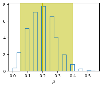
In this example, we have flipped enough to establish \(p\pm 0.2\) with 95% confidence, but not \(p \pm 0.1\).

2. Curve Fitting

While in principle you can do this part with standard least-squares regression, I recommend you use the MCMC emcee package or something similar in your language of preference. It will be quite difficult to get the proper credible interval using least-squares techniques alone.

Consider the model

\[\begin{gather*} y = (0.5+t)^{a} + (0.5+t)^{b} + \epsilon \end{gather*}\]

where the errors \(\epsilon\) are expected to be normal with standard deviation \(\sigma\). Fit the model to the following data and report the 68% and 95% confidence intervals for each parameter, marginalizing over the other parameter. Note that this model is degenerate under the exchange \(a \leftrightarrow b\). Use uniform priors that ensure \(a>0\) and \(b<0\). Follow the approach in Parameter Fitting, first doing a simple curve fit, then doing a full Bayesian analysis.

Show code cell source

Hide code cell source

from IPython.display import display, Math
import numpy as np, matplotlib.pyplot as plt
import corner
import uncertainties
import emcee
from scipy.optimize import curve_fit

# Parameter values: these are the "truths" in our simulations
a = 1.2
b = -1.5

# Here is the function we are fitting.  We use the true values as the defaults
def f(t, a=a, b=b):
    return (0.5+t)**a + (0.5+t)**b

T = 5.0
Nt = 11  # Number of data points.

ts = np.linspace(0, T, Nt)
sigma = 1.0                          # Constant errors +-1
rng = np.random.default_rng(seed=2)  # Always seed so you can reproduce results

# Simulate some gaussian measurement errors
eps = rng.normal(scale=sigma, size=Nt)
xdata = ts
ydata = f(ts) + eps
yerrs = np.ones(Nt) * sigma

print(f"{ts=}")
print(", ".join(f"{uncertainties.ufloat(y, dy):S}" for y, dy in zip(ydata, yerrs)))

# Plot the data
fig, ax = plt.subplots(figsize=(4, 3))
t = np.linspace(0, T)
ax.plot(t, f(t))
ax.set(xlabel="$t$ [s]", ylabel="$z$ [m]");
ax.errorbar(xdata, ydata, yerr=yerrs, fmt='+k');

ts=array([0. , 0.5, 1. , 1.5, 2. , 2.5, 3. , 3.5, 4. , 4.5, 5. ])
3.5(1.0), 1.5(1.0), 1.8(1.0), 0.2(1.0), 5.1(1.0), 5.1(1.0), 4.3(1.0), 6.2(1.0), 6.5(1.0), 6.4(1.0), 8.8(1.0)

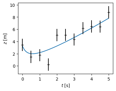
xdata = np.array([0.0, 0.5, 1.0, 1.5, 2.0, 2.5, 3.0, 3.5, 4.0, 4.5, 5.0])
ydata = np.array([3.5, 1.5, 1.8, 0.2, 5.1, 5.1, 4.3, 6.2, 6.5, 6.4, 8.8])
yerrs = np.array([1.0, 1.0, 1.0, 1.0, 1.0, 1.0, 1.0, 1.0, 1.0, 1.0, 1.0])

As a check, with the full analysis you should find the following 95% CI for \(b\):

\[\begin{gather*} b = -1.5^{+1.2}_{-0.7} \end{gather*}\]

(These are 2.5%, 50%, and 97.5% percentiles.) In contrast, naïvely using a least squares approach gives \(b = -1.7(5)\), which underestimates the errors and bias.

3. Arrival Time

Consider measuring photons from a distance supernova explosion. Suppose the probability density of observing photons is a decaying exponential

\[\begin{gather*} p(t) \propto \begin{cases} e^{-t/\tau} & t > t_0,\\ 0 & \text{otherwise}. \end{cases} \end{gather*}\]

I.e., before the time \(t_0\) of the arrival of the first photon, there is no chance of seeing one, then the probability decays exponentially. Assuming that the decay constant \(\tau\) is known, we measure all times in this unit, so set \(\tau = 1\). Suppose you detect three photons, one each at times \(t \in \vect{t} = [12, 14, 16]\). Your goal is to determine an estimate of \(t_0\).

First do this using a Bayesian estimate with a uniform prior to obtain the posterior

\[\begin{gather*} p(t_0 | \vect{t}) = \begin{cases} \frac{3}{\tau}e^{6}e^{3(t_0/\tau - 14)} & t_0 < 12\tau\,,\\ 0 & \text{otherwise}. \end{cases} \end{gather*}\]

Now consider the standard statistical technique. Check the following results numerically.

import numpy as np
rng = np.random.default_rng(seed=2)
Ns = 10000
t0 = 12
tau = 1.2
ts = t0 + rng.exponential(scale=tau, size=Ns)

fig, ax = plt.subplots(figsize=(3, 2), constrained_layout=True)
ax.hist(ts, bins=int(np.sqrt(Ns)), density=True)
ax.set(xlabel="$t$", ylabel="$p(t)$");

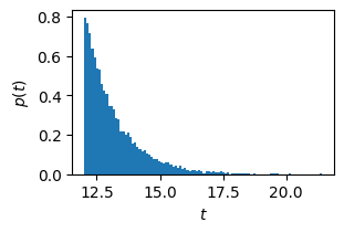
1. The proper normalization for \(p(t)\) is

   \[\begin{gather*} p(t) = \Theta(t-t_0)e^{(t_0 - t)/\tau}. \end{gather*}\]

   Note you can use numpy.random.Generator.exponential() to generate a random variable with this distribution as shown in the margin.

2. Check that for photons following this distribution, the mean is \(\braket{t} = t_0 + \tau\).

3. Using \(\hat{t} = \braket{t} - \tau\) as an estimator for \(t_0\), from our data we have mean \(\braket{t} = 14\tau\), hence, correcting for the bias, we have the estimate \(t_0 = 14-1 = 13\).

4. One can show with a bit of work that the distribution of the estimator \(\hat{t} = \braket{t} - \tau\) for \(N\) measurements is

   \[\begin{gather*} p(\hat{t}|t_0) = \frac{1}{\tau} \frac{N^N}{(N-1)!}\theta(y)y^{N-1}e^{-Ny}\,, \qquad y = \frac{\hat{t} - t_0}{\tau} + 1. \end{gather*}\]

   Check this numerically for \(N=3\) photons by simulating data.

5. Show that the cumulative distribution for \(N=3\) measurements has the form

   \[\begin{gather*} C(\hat{t}|t_0) = 1 - e^{-3y}(1+3y + \tfrac{9}{2}y^2). \end{gather*}\]

   Use this to show that \(y \in [0.15, 1.83]\) is a 90% highest-probability density confidence interval (CI). (Simply plot these limits an verify that 1) the area under the curve \(p(\hat{t}|t_0)\) is 90% and 2) that this is the region containing 90% of the events with highest probability density.)

   Thus, one would be tempted to claim from this data that with 90% confidence

   \[\begin{gather*} \frac{t_0}{\tau} = 13 \pm 0.85. \end{gather*}\]

   Notice that the observation of a photon at time \(t=12\) means that \(t_0 < 12\): the 90% CI lies completely in the impossible region! Explain what is going on?

4. Generating Random Data

Hint: to get started, you might first consider the following simpler cases:

\[\begin{gather*} p_Y(y) = \begin{cases} \frac{1}{L} & 0 \leq y \leq L\\ 0 & \text{otherwise} \end{cases},\\ p_Y(y) = \begin{cases} \frac{2y}{L^2} & 0 \leq y \leq L\\ 0 & \text{otherwise} \end{cases}. \end{gather*}\]

Suppose you have a pseudo-random number generator like numpy.random.default_rng() that can generate samples \(\{x_i\}\) uniformly distributed in the interval \(x\in [0, 1]\): i.e., with PDF

\[\begin{gather*} p_X(x) = \begin{cases} 1 & 0 \leq x \leq 1\\ 0 & \text{otherwise} \end{cases} \end{gather*}\]

How can you use this to generate samples \(\{y_{i}\}\) distributed with the following PDF:

\[\begin{gather*} p_Y(y) = \begin{cases} 6y(1-y) & 0 \leq y \leq 1\\ 0 & \text{otherwise} \end{cases} \end{gather*}\]

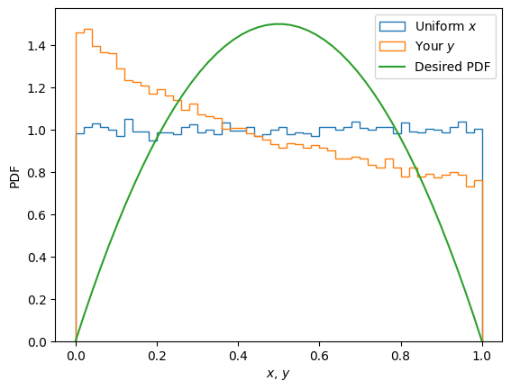
Test your answer by making a histogram with code like this:

import numpy as np, matplotlib.pyplot as plt

rng = np.random.default_rng(seed=2)

Ns = 100000  # Number of samples
x = rng.random(size=Ns)  # Uniform

y = ((1+x)**2-1)/3  ##### WRONG! Implement your answer here.

fig, ax = plt.subplots()
kw = dict(density=True, bins=50,histtype='step')
ax.hist(x, label="Uniform $x$", **kw)
ax.hist(y, label="Your $y$", **kw)

y_ = np.linspace(0, 1)
p_Y = np.where(np.logical_and(0 < y_, abs(y_) < 1), 
               6*y_*(1-y_), 0)
ax.plot(y_, p_Y, label="Desired PDF")
ax.legend()
ax.set(xlabel="$x$, $y$", ylabel="PDF");