11. Complex Analysis

11. Complex Analysis#

Complex analysis provides a powerful framework unifying the following concepts, which are extremely useful for physical applications.

Contour integration and Cauchy’s residue theorem: These provide a powerful approach for computing many difficult integrals of interest in physics, such as the following from Assignment 2: Mathematical Preliminaries:

\[\begin{gather*} \int_0^{\infty}\frac{\sin x}{x}\d{x}. \end{gather*}\]

These approaches rely on the concepts of analytic functions (functions defined from their power series – equivalent to holomorphic functions in complex analysis) and analytic continuation, zeros, poles, branch cuts, and essential singularities.

Conformal maps: Transformations that preserve angles can often help solve problems. The real and imaginary parts of holomorphic functions are harmonic functions, which provide solutions to Laplace’s equation. Conformal maps preserve this property, allowing one to find simple symmetric solutions to e.g. the wave equation, then transform them to more complicated boundaries or geometries. On very interesting example is the using the Joukowsky transform to take the symmetric solution for laminar flow past a cylinder into the to flow across the Joukowsky airfoil.

Analytic Functions #

Recall that many functions can be defined in terms of a power series:

\[\begin{gather*} f(x) = \sum_{n=0}^{\infty} c_{n} x^{n}, \end{gather*}\]

with some range of convergence \(-R < x < R\). By expanding about different points, one can often extend the definition of the function through a sequence of converging power series. This is called analytic continuation.

Example: Analytic continuation of a real function \(f(x) = 1/(1-x)\).

Consider a geometric series

\[\begin{gather*} f(x) = \sum_{n=0}^{\infty} x^{n} = \frac{1}{1-x}, \qquad -1 < x < 1. \end{gather*}\]

This series converges absolutely to a \(\mathcal{C}^{\infty}\) function on the open interval \(x \in (-1, 1)\), but the function itself seems like it should be defined for \(x \leq -1\). We can try performing a expanding about \(x_0=-\tfrac{1}{2}\):

\[\begin{gather*} f(x) = \sum_{n=0}^{\infty}\left(\frac{2}{3}\right)^{n+1}(x+\tfrac{1}{2})^{n} = \frac{2}{3}\sum_{n=0}^{\infty}\left(\frac{2x+1}{3}\right)^{n}\\ = \frac{2}{3}\frac{1}{1-\frac{2x+1}{3}} = \frac{1}{1-x}, \qquad -1 < \frac{2x+1}{3} < 1. \end{gather*}\]

This now converges absolutely on the open interval \(x \in (-2, 1)\). Continuing, we can expand about other points \(x_0<0\) to obtain

\[\begin{gather*} f(x) = \sum_{n=0}^{\infty}\frac{1}{(1-x_0)^{n+1}}(x-x_0)^n = \frac{1}{1-x_0}\sum_{n=0}^{\infty}\left(\frac{x-x_0}{1-x_0}\right)^n\\ = \frac{1}{1-x_0}\frac{1}{1-\frac{x-x_0}{1-x_0}} = \frac{1}{1-x}, \qquad -1 < \frac{x-x_0}{1-x_0} < 1, \end{gather*}\]

which converges absolutely on the open interval \(x \in (2x_0-1, 1)\). Thus, we can analytically continue the function defined by the original series to \(x \in (-\infty, 1)\). As [Needham, 2023] states, from the perspective of real analysis, the interval of convergence is quite mysterious, but notice that it is always symmetric about \(x_0\):

\[\begin{gather*} x-x_0 \in (-R, R), \qquad R = 1-x_0. \end{gather*}\]

This “radius of convergence” \(R\) has a beautifully simple explanation in the complex plane – it is the distance to the nearest pole: \(x=1\) in this case.

This explains the mystery [Needham, 2023] of the following series:

\[\begin{gather*} G(x) = \frac{1}{1-x^2} = \sum_{n=0}^{\infty}x^{2n}, \qquad H(x) = \frac{1}{1+x^2} = \sum_{n=0}^{\infty}(-1)^n x^{2n}. \end{gather*}\]

Both have the same interval of convergence: \(x\in (-1, 1)\). This makes sense for \(G(x)\) which has poles at \(x = \pm 1\), but \(H(x)\) is perfectly smooth.

This can be easily extended to the complex plane:

\[\begin{gather*} f(z) = \sum_{n=0}^{\infty} c_n z^{n}, \qquad z = x + \I y. \end{gather*}\]

For example,

\[\begin{gather*} e^{z} = e^{x + \I y} = e^{x}e^{\I y} = e^{x}(\cos y + \I \sin y). \end{gather*}\]

Do It! Similarly compute \(\sin{z}\), \(\cos{z}\), \(\sinh{z}\), \(\cosh{z}\), and \(\ln{z}\).

For \(\sin{z}\), \(\cos{z}\), etc. we use Euler’s identity \(e^{z} = \cos z + \I \sin z\). We first note that

\[\begin{gather*} \sinh z = \frac{e^{z} - e^{-z}}{2} = \I\frac{e^{\I (z/\I)} - e^{-\I (z/\I)}}{2\I} = \I \sin \frac{z}{\I} = -\I \sin(\I z)\\ \cosh z = \frac{e^{z} + e^{-z}}{2} = \frac{e^{\I (z/\I)} + e^{-\I (z/\I)}}{2} = \cos \frac{z}{\I} = \cos(\I z). \end{gather*}\]

I remember these as follows, without any minus signs

\[\begin{gather*} \cos \I z = \cosh z, \qquad \sin \I z = \I \sinh z,\\ \cosh \I z = \cos z, \qquad \sinh \I z = \I \sin z. \end{gather*}\]

We also have the addition formulae, which follow from expanding \(e^{a+b} = e^{a}e^{b}\):

\[\begin{gather*} \sin(x+y) = \sin{x}\cos{y} + \cos{x}\sin{y}, \\ \cos(x+y) = \cos{x}\cos{y} - \sin{x}\sin{y}, \\ \sinh(x+y) = \sinh{x}\cosh{y} + \cosh{x}\sinh{y}, \\ \cosh(x+y) = \cosh{x}\cosh{y} + \sinh{x}\sinh{y}. \end{gather*}\]

Now we have

\[\begin{align*} \sin z &= \sin(x+\I y) = \cos(\I y)\sin x + \sin(\I y)\cos x\\ &= \cosh y \sin x + \I\sinh y \cos x,\\ \cos z &= \cos(x+\I y) = \cos(\I y)\cos x - \sin(\I y)\sin x\\ &= \cosh y \cos x - \I\sinh y \sin x,\\ \sinh z &= \sinh(x+\I y) = \cosh(\I y)\sinh x + \sinh(\I y)\cosh x\\ &= \cos y \sinh x + \I\sin y \cosh x,\\ \cosh z &= \cosh(x+\I y) = \cosh(\I y)\cosh x + \sinh(\I y)\sinh x\\ &= \cos y \cosh x + \I\sin y \sinh x. \end{align*}\]

For \(\ln z\) we define \(w = \ln z\) so that \(z = e^w\). For this, polar form is better for \(z = re^{\I\theta}\):

\[\begin{gather*} \ln z = \ln (re^{\I(\theta + 2\pi n)}) = \ln r + \I (\theta + 2\pi n) = \ln\sqrt{x^2+y^2} + \I \tan^{-1}\frac{y}{x} + 2\pi \I n. \end{gather*}\]

In the complex plane, analytic functions can be expressed in terms of \(z\) only: e.g. \(z^2\), \(e^z\), \(\sin(z)\). [Hassani, 2013] formalizes this in Box 10.2.3: If a function is complex analytic, then, after substituting \(x = (z+z^*)/2\) and \(y=(z-z^*)/2\), it will be independent of \(z^*\).

Multifunctions#

Consider the behaviour of \(z \mapsto w = e^{z}\) shown below (from [Needham, 2023]).

Show code cell source

Hide code cell source

# Code to produce figure 2.19 from [Needham:2023]
from matplotlib import patches
from scipy.interpolate import CubicSpline


class Conformal:
    """Demonstration of a conformal map."""
    
    x0, y0 = 1, 5     # Initial grid is [-x0, x0] × [0, y0] before scaling
    Nx = 11           # Number of gridlines along x
    shift, scale = 0j, 1,  # Shift and scale before f(z).
    resolution = 100  # Number of points to add to make lines curved.
    
    # Plotting parameters for various elements
    grid_kw = dict(lw=0.5, c='k', ls='-')

    # Various shapes
    T = np.array([1+0j, 2+0j, 2+2j, 3+2j, 3+3j, 0+3j, 0+2j, 1+2j])
    L = np.array([1+0j, 2+0j, 2+2j, 3+2j, 3+3j, 1+3j])
    T_scale = 1
    T_shift = 1+21j
    T_args = dict(fc='C0')

    L_scale = T_scale
    L_shift = T_shift
    L_args = T_args

    def __init__(self, **kw):
        for key in kw:
            if not hasattr(self, key):
                raise ValueError(f"Unknown {key=}")
            setattr(self, key, kw[key])
        self.init()
    
    def init(self):
        self.dx = 2 * self.x0 / (self.Nx - 1)
        self.Ny = int(np.ceil(self.y0/self.dx))
        self.y0 = self.dx * self.Ny
    
    def f(self, z):
        """The conformal transformation."""
        return z
        
    def _f(self, z):
        """Private version subclasses can change."""
        return self.f(z)
    
    def fun(self, z):
        """Return f((z + shift)*scale)."""
        return self._f((np.asarray(z) + self.shift)*self.scale)
        
    def transform(self, z):
        """Return transformed coordinates (x, y)."""
        fz = self.fun(z)
        return fz.real, fz.imag
        
    def interpolate(self, zs, resolution=None, closed=True):
        """Return a new path with intermediate points added to each segment."""
        if resolution is None:
            resolution = self.resolution
        lam = np.arange(resolution) / resolution
        if closed:
            z0s = zs
            z1s = np.concatenate([zs[1:], zs[:1]])
        else:
            z0s = zs[:-1]
            z1s = zs[1:]
        Zs = [(1-lam)*z0 + lam*z1 for z0, z1 in zip(z0s, z1s)]
        if not closed:
            Zs.append([zs[-1]])
        return np.concatenate(Zs)

    arrow_kw = dict(length_includes_head=True,
                    overhang=0.4,
                    color='k')
    # Arrows and dots
    def draw_arrows(self, zs, N=1, length=0.2):
        """Draws N arrows equally spaced along zs.

        Equally spaced means equally along the index of zs.
        """
        ax = self._ax
        spl = CubicSpline(np.linspace(0, 1, len(zs)), zs)
        lams = np.linspace(0, 1, N+1)[1:]
        for lam in lams:
            z, dz = spl(lam), spl.derivative()(lam)
            dz *= length/abs(dz)
            z0 = z-dz

            arrow = patches.FancyArrow(
                z0.real, z0.imag, dz.real, dz.imag,
                head_width=length, head_length=length,
                **self.arrow_kw)
            ax.add_patch(arrow)

    def draw_line(self, z0, z1, ls='-', c='k', Narrows=0,
                  marker=None, ms=5.0, mfc='w', markeredgewidth=0.2,
                  **kw):
        """Draw a line from z0 to z1 with N arrows."""
        ax = self._ax
        if z0 is not None and z1 is not None:
            zs = self.interpolate([z0, z1], closed=False)
            ax.plot(*self.transform(zs), ls=ls, c=c, **kw)
        if marker:
            ax.plot(*self.transform([z1]), c=c, 
                    marker=marker, ms=ms, mfc=mfc, markeredgewidth=markeredgewidth,
                    zorder=100)

            # Currently a fudge factor so arrows do not overlap maerker.
            # Ideally we will  convert from ms
            dz = z1-z0
            dz *= 0.2 * self.dx / abs(dz)
            zs = self.interpolate([z0, z1-dz], closed=False)
        if Narrows > 0:
            self.draw_arrows(self.fun(zs), N=Narrows)

    def draw_grid(self):
        ax = self._ax

        # Main grid
        x0, y0 = self.x0, self.y0
        X = np.linspace(-x0, x0, self.Nx)[:-1]
        Y = np.arange(self.Ny+1) * self.dx
        x = np.linspace(-x0, x0, self.resolution)
        y = np.linspace(0, y0, self.resolution)

        X, y = np.meshgrid(X, y, indexing='ij')
        x, Y = np.meshgrid(x, Y, indexing='ij')
        ax.plot(*self.transform(x+1j*Y), **self.grid_kw)
        ax.plot(*self.transform(X.T + 1j*y.T), **self.grid_kw)

        # Grey patch
        P = np.array([-x0, 0, 0+y0*1j, -x0 + 1j*y0])
        P = self.interpolate(P, closed=True)
        P = self.fun(P)
        ax.add_patch(patches.Polygon(np.transpose([P.real, P.imag]), color='lightgrey'))
        ax.set(aspect=1)
    
    def draw_T(self):
        ax = self._ax
        T = self.interpolate(self.T, resolution=10, closed=True)
        T = (T * self.T_scale + self.T_shift) * self.dx
        ax.add_patch(patches.Polygon(np.transpose(self.transform(T)), **self.T_args))

    def draw_L(self):
        ax = self._ax
        L = self.interpolate(self.L, resolution=10, closed=True)
        L = (L * self.L_scale + self.L_shift) * self.dx
        ax.add_patch(patches.Polygon(np.transpose(self.transform(L)), **self.L_args))
    
    def draw(self, ax=None, z=1-0.5j):
        """Demonstrates a conformal map."""
        if ax is None:
            fig, ax = plt.subplots()
        self._ax = ax

        self.draw_grid()
        self.draw_L()

        # The lines
        x0 = self.x0
        for s in [2, 4]:
            self.draw_line(-x0+0j, x0+1j*s*x0, ls='-', c='k')
        
        self.draw_line(z, z - 2*self.x0, Narrows=4, ls='-')
        self.draw_line(z, z+2j*np.pi, ls='--', dashes=(8, 4), lw=1, Narrows=4,
                       marker='o')
        
        # Some extra points
        zs = np.array([0.0, z])
        ax.plot(*self.transform(zs), 'ok', mfc='w', markeredgewidth=0.2)

        return z

f = np.exp

map0 = Conformal()
map1 = Conformal(f=f)

fig, axs = plt.subplots(1, 2, width_ratios=(1, 3), figsize=(6, 4))

ax = axs[0]
ax.axvline(0, c='k', lw=0.3)
ax.axhline(0, c='k', lw=0.3)

z1 = map0.draw(ax=ax)

kw = dict(xytext=(1, 0), textcoords='offset fontsize', va='center')
ax.annotate("$z$", (z1.real, z1.imag), **kw)
ax.annotate("$z+2\pi\mathrm{I}$", (z1.real, z1.imag + 2*np.pi), **kw)
ax.annotate("$0$", (0, 0), **dict(kw, xytext=(-0.3, -0.3), ha='right', va='top'))

ax = axs[1]
map1.draw(ax=ax)
ax.annotate("$1$", (1, 0), **dict(kw, xytext=(0, -0.5), ha='center', va='top'))
ax.annotate("$w$", (f(z1).real, f(z1).imag), 
                   **dict(kw, xytext=(1, -1), ha='center', va='center'))
plt.suptitle("Effect of the mapping $e^z$")
for ax in axs:
    ax.set_axis_off()

_images/6e7b0c206e8546804d902fd34fd04138062a2292287a4e1fc50ee9c1ce21a2f7.png

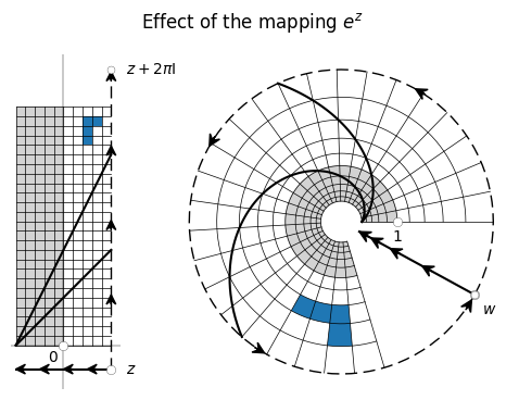
Notice that it takes maps a strip \((-\infty, \infty)\times [y, y+2\pi \I]\) into the entire plane \(\mathbb{C} \equiv \mathbb{R}^2\). Specifically, the points with \(x\leq 0\) get mapped into the unit ball \(r\leq 0\), while the points \(x >0\) are mapped to the outside disk. Different strips in the \(y\) direction of width \(2\pi\) will be mapped on top of each other. Hence, the inverse function \(\ln z\) must be multi-valued – a multifunction as [Needham, 2023] calls them.

To see this, consider \(\ln z\) where \(z = re^{\I\theta} \equiv re^{\I\theta + 2\pi \I n}\) since \(e^{2\pi \I n} = 1\) where \(n\) is an integer. Thus:

\[\begin{gather*} \ln z = \ln r + \I (\theta + 2\pi n) \end{gather*}\]

where the integer \(n\) specifics which branch of the function we are “on”. To be definite, one usually defines the following functions with capital letters to denote that they yield the principal branch or principal value:

\[\begin{gather*} \DeclareMathOperator{\Log}{Log} \DeclareMathOperator{\Arg}{Arg} z = r e^{\I\theta},\qquad \abs{z} = r, \qquad \Arg(z) = \theta \in (-\pi, \pi],\qquad \Log(z) = \ln\,\abs{z} + \I \Arg(z). \end{gather*}\]

You should already be familiar with this idea: for example both \(+1\) and \(-1\) square to \(1\), so you should be familiar with \(z^{1/2}\) being a multifunction with two branches.

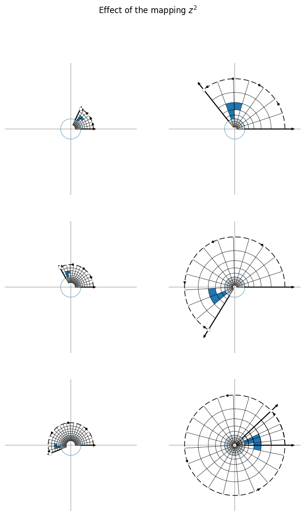
_images/ac32f69849890113bbd24bdb08bef90b877f7897d229db34db2ab69b022c74d5.png

Since the angle doubles, the map \(z\mapsto z^2\) effects a double cover of the plane. Similarly \(z^n\) for positive integer \(z\) will effect an \(n\)-cover.

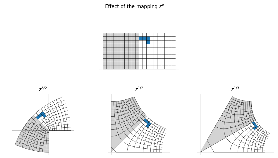
Do It! Compute all the values of \(w = z^k\) for real \(k\).

Using all branches of \(\ln\), we have:

\[\begin{gather*} \ln w = k \ln x = k (\Log z + 2\pi \I n),\qquad w = e^{k\ln z} = e^{k\Log z + 2\pi \I n k} = \abs{z}^{k} e^{\I k(\Arg z + 2\pi n)}. \end{gather*}\]

If \(k = p/q\) is rational with \(p\) and \(q\) relatively prime, then there will be \(q\) distinct branches or roots. If \(k\) is irrational, then there will be infinitely many branches for each \(n\).

Note that this makes the notion of \(e^{z}\) somewhat uncomfortable since, \((2.718\dots)^{z}\) is a multifunction with possibly infinitely many branches, depending on the value of \(z\)! We follow [Needham, 2023] and define \(e^{z}\) to be the single-valued exponential mapping, not the multifunction \((2.718\dots)^{z}\).

Clausen’s Paradox: \((e^{a})^{b} = e^{ab} \Rightarrow 1=e^{-2\pi}\).

We know that \(e^{2\pi \I} = 1\), therefore \((e^{2\pi \I})^{\I} = 1^\I = 1\), but if \((e^{a})^{b} = e^{ab}\), then we must conclude that \((e^{2\pi \I})^{\I} = e^{-2\pi} = 1\), which is rather absurd.

One must be careful with complex powers. The multifunction \(z^k\) is defined to be

\[\begin{gather*} z^{k} = e^{k \ln z} = e^{k(\Log z + 2\pi \I n)}, \end{gather*}\]

but it does not follow that \((e^{a})^{b} = e^{ab}\) as it does for real numbers. Instead, we should let \(z=e^{a}\) and \(k=b\) to get

\[\begin{gather*} (e^{a})^{b} = e^{b \ln e^{a}} = e^{b (a + 2\pi \I n)}. \end{gather*}\]

Applying this to our original expression, we have

\[\begin{gather*} (e^{2\pi \I})^{\I} = e^{\I (2\pi \I + 2\pi \I n)} = e^{-2\pi (1+n)}. \end{gather*}\]

This is \(1\) for the appropriate branch \(n=-1\). In summary, when discussing multifunctions, one should restrict oneself carefully to use the definitions like \(z^{k} = e^{k \ln z} = e^{k(\Log z + 2\pi \I n)}\).

Do It! Show that the branches of \(k^{z}\) are unrelated.

Follow [Needham, 2023] Ex. 29 in §2.9 and show that the “branches” of \(k^{z}\) are

\[\begin{gather*} k^{z} = e^{l_n z}, \qquad l_n = (\Log k + 2\pi \I n), \end{gather*}\]

but that each of these branches is “unrelated” in the sense that, if you start on one branch, you cannot get to another by moving continuously (analytic continuation). Thus, the multifunction \(k^{z}\) has no branch cuts, but should be thought of as a collection \(\{\dots, e^{l_{-1}z}, e^{l_0z}, e^{l_1z}, \dots\}\) of unrelated single-valued functions.

Derivatives: Cauchy-Riemann Conditions#

The first idea is to extend the notion of the derivative to complex-valued functions. Proceeding in analogy from calculus, we would like

\[\begin{gather*} \diff{f(z)}{z} = \lim_{h \rightarrow 0} \frac{f(z+h) - f(z)}{h}. \end{gather*}\]

The difficulty now is that we must consider \(h\in \mathbb{C}\) as complex. Thus, we can write, for real \(h\):

\[\begin{gather*} \diff{f(z)}{z} = \lim_{h \rightarrow 0} \frac{f(z+hw) - f(z)}{hw}, \qquad w = e^{\I\phi}. \end{gather*}\]

This gives the directional derivative along the direction \(w=e^{\I\phi}\). For such a derivative to make sense, the result must be independent of \(w\), which leads to the Cauchy-Riemann equations:

\[\begin{gather*} \pdiff{u}{x} = \pdiff{v}{y}, \qquad \pdiff{u}{y} = -\pdiff{v}{x}. \end{gather*}\]

Do It! Derive the Cauchy-Riemann condition.

Compute and equate the directional derivatives for \(f(x, y) = u(x, y) + \I v(x, y)\) along \(w = 1\) (along the real axis \(\partial_x\)) and \(w=\I\) (along the imaginary axis \(\partial_y/\I\)):

\[\begin{gather*} \underbrace{\pdiff{u}{x} + \I\pdiff{v}{x}}_{\partial_x f(z)} = \underbrace{-\I\pdiff{u}{y} + \pdiff{v}{y}}_{\partial_y f(z)/\I}. \end{gather*}\]

The Cauchy-Riemann conditions follow after equating the real and imaginary parts.

Do It! Prove these mean that \(f\) is independent of \(z^*\).

Treating \(z\) and \(z^*\) as independent, we express

\[\begin{gather*} x = \frac{z+z^*}{2}, \qquad y = \frac{z - z^*}{2\I},\\ f(z, z^*) = u\left(\frac{z+z^*}{2}, \frac{z-z^*}{2\I}\right) + \I v\left(\frac{z+z^*}{2}, \frac{z-z^*}{2\I}\right),\\ \pdiff{f(z, z^*)}{z^*} = \frac{\pdiff{u}{x} + \I \pdiff{u}{y} + \I \Bigl(\pdiff{v}{x} + \I\pdiff{v}{y}\Bigr)}{2} = \frac{\pdiff{u}{x} - \pdiff{v}{y} + \I \Bigl(\pdiff{u}{y} + \pdiff{v}{x}\Bigr)}{2}. \end{gather*}\]

Hence, the Cauchy-Riemann conditions are satisfied iff

\[\begin{gather*} \pdiff{f(z, z^*)}{z^*} = 0, \end{gather*}\]

i.e. if \(f\) is independent of \(z^*\).

Functions that satisfy these Cauchy-Riemann equations in a neighbourhood of a point \(z_0\) are said to be complex analytic (or just analytic) at \(z_0\). Complex analytic functions are also called holomorphic functions.

This has some interesting consequences for derivatives. Independence of direction means

\[\begin{gather*} f'(z) = \underbrace{\overbrace{\pdiff{f}{x}}^{f_{,x}}}_{\pdiff{f}{x}/\pdiff{z}{x}} = \underbrace{-\I \overbrace{\pdiff{f}{y}}^{f_{,y}}}_{\pdiff{f}{y}/\pdiff{z}{y}}. \end{gather*}\]

\[\begin{gather*} \end{gather*}\]

Since \(f'(z)\) is analytic at the same places as \(f(z)\), we can repeat this:

\[\begin{gather*} f''(z) = f_{,xx} = -f_{,yy} = -\I f_{,xy}. \end{gather*}\]

You can use and rearrange these as needed.

Saddle points: the Hessian of \(\Re f\) and \(\Im f\).

As an example of these types of manipulations, consider the Hessian matrix of \(u(x, y)\) and \(v(x, y)\):

\[\begin{gather*} \mat{U} = \begin{pmatrix} u_{,xx} & u_{,xy}\\ u_{,yx} & u_{,yy} \end{pmatrix}, \qquad \mat{V} = \begin{pmatrix} v_{,xx} & v_{,xy}\\ v_{,yx} & v_{,yy} \end{pmatrix}. \end{gather*}\]

These are useful for the Saddle-point Approximation where the orientation of the saddle is given by the eigenvectors of these matrices. We suspect that this information is codified in \(f''(z)\), but how? Consider the action of \(f''(z)\):

\[\begin{gather*} f''(z)z = (u_{,xx} + \I v_{,xx})(x+\I y) = (u_{,xx}x - v_{,xx}y) + \I(v_{,xx}x + u_{,xx}y). \end{gather*}\]

This last expression can be manipulated into a useful form using the Cauchy-Riemann equations:

\[\begin{align*} u_{,x} &= v_{,y}, & u_{,xx} &= v_{,xy} = v_{,yx} = -u_{,yy}, \\ u_{,y} &= -v_{,x}, & v_{,xx} &= u_{,xy} = u_{,yx} = -v_{,yy}. \end{align*}\]

Thus, let \((x, y)^T\) be an eigenvector of \(\mat{U}\) or \(\mat{V}\). We first express this, then use these manipulations to find a relevant form of \(f'' z\):

\[\begin{align*} \mat{U}\begin{pmatrix} x\\ y \end{pmatrix} &= \begin{pmatrix} u_{,xx}x + u_{,xy}y\\ u_{,xy}x + u_{,yy}y \end{pmatrix} =\lambda\begin{pmatrix} x\\ y \end{pmatrix} & \mat{V}\begin{pmatrix} x\\ y \end{pmatrix} &= \begin{pmatrix} v_{,xx}x + v_{,xy}y\\ v_{,xy}x + v_{,yy}y \end{pmatrix} =\lambda\begin{pmatrix} x\\ y \end{pmatrix},\\ f''(z)z &= (u_{,xx}x + u_{,xy}y) - \I(u_{,xy}x + u_{,yy}y) & f''(z)z &= (v_{,xy}x + v_{,yy}y) + \I(v_{,xx}x + v_{,xy}y),\\ &= \begin{pmatrix} 1 & -\I \end{pmatrix} \mat{U}\begin{pmatrix} x\\ y \end{pmatrix} = \lambda(x - \I y) = \lambda z^*, & &= \begin{pmatrix} \I & 1 \end{pmatrix} \mat{V}\begin{pmatrix} x\\ y \end{pmatrix} = \lambda(\I x + y) = \I\lambda z^*. \end{align*}\]

Thus, we arrive at the somewhat non-trivial relationships for eigenvectors of the real and imaginary Hessians respectively:

\[\begin{gather*} f''(z) z = \lambda z^*, \qquad f''(z) z = \I \lambda z^*. \end{gather*}\]

Consider these in polar coordinates:

\[\begin{gather*} f''(z) = Re^{\I\Phi}, \qquad z = re^{\I\phi}, \qquad f''(z) z = Rre^{\I(\Phi + \phi)}, \qquad \lambda z^* = \lambda r e^{-\I\phi}. \end{gather*}\]

Hence, for \(\mat{U}\) and \(\mat{V}\) respectively, we have

\[\begin{align*} \lambda_{U} &= R, & \phi_{U} &= \frac{-\Phi}{2}, & \lambda_{U} &= -R, & \phi_{U} &= \frac{\pi - \Phi}{2}, \\ \lambda_{V} &= R, & \phi_{V} &= \frac{-\Phi + \tfrac{\pi}{2}}{2}, & \lambda_{V} &= -R, & \phi_{V} &= \frac{\pi -\Phi + \tfrac{\pi}{2}}{2},\\ \phi_{V} &= \phi_{U} + \frac{\pi}{4}. \end{align*}\]

This is the content of Eq. (3-82) in [Mathews and Walker, 1970] and Eq. (12.103) in [Arfken et al., 2013]. They proceed more directly, expanding \(f(z)\) to second order:

\[\begin{gather*} f(z) = f(z_0) + f'(z_0)(z-z_0) + \frac{f''(z_0)}{2!}(z-z_0)^2 + \dots. \end{gather*}\]

Now let \((z-z_0) = x + \I y = re^{\I\phi}\) and \(f''(z_0) = Re^{\I\Phi}\):

\[\begin{gather*} \frac{f''(z_0)(z-z_0)^2}{Rr^2} = e^{\I(\Phi + 2\phi)} = \cos(\Phi + 2\phi) + \I \sin(\Phi + 2\phi). \end{gather*}\]

The eigenvectors for \(U\) and \(V\) respectively correspond to the directions of maximal ascent and descent for the real and imaginary portions. Thus

\[\begin{gather*} \Phi + 2\phi_{U} = \pi n, \qquad \Phi + 2\phi_{V} = \pi n + \frac{\pi}{2},\\ \phi_{U} = \frac{\pi n - \Phi}{2}, \qquad \phi_{V} = \frac{\pi n + \tfrac{\pi}{2} - \Phi}{2}. \end{gather*}\]

The moral of this calculation is thus: the Cauchy-Riemann equations admit for many simplifications, but the most direct approach generally proceeds by directly working with the analytical structure – Taylor series, etc.

Conformal Maps and Harmonic Functions#

Consider how an analytic function \(f(z)\) behaves near \(z_0\):

\[\begin{gather*} f(z) = \underbrace{f(z_0)}_{b} + \underbrace{f'(z_0)}_{a}(z-z_0) + O\Bigl((z-z_0)^2\Bigr). \end{gather*}\]

This means that, locally, \(f(z)\) acts like \(z \mapsto az + b\) where \(a, b\in\mathbb{C}\) are complex numbers. This means that locally, analytic functions are amplitwists: the factor \(a\) scales and rotates the function, while the constant \(b\) shifts the function.

To see this, use polar coordinates:

\[\begin{gather*} z = re^{\I\theta}, \qquad a = f'(z_0) = se^{\I\phi}, \qquad az = (sr)e^{\I(\theta+\phi)}. \end{gather*}\]

This is a combination of an “amplification” scaling the radius by a factor \(s\) and a “twist”, rotating the region of the plane by \(\phi\). Significantly, such transformations preserve angles: hence an analytic functions \(f: \mathbb{C}\mapsto\mathbb{C}\) locally defines a conformal map. This property has many uses, as will be discussed below.

As a consequence of the Cauchy-Riemann equations, the real and imaginary parts of analytic functions are harmonic functions, meaning that they satisfy Laplace’s equation:

\[\begin{gather*} f(z) = u(x, y) + \I v(x, y), \qquad \nabla^2 u(x, y) = \nabla^2 v(x, y) = 0. \end{gather*}\]

Do It! Prove this.

Compute the partials, then replace \(u_{,x} \leftrightarrow v_{,x}\) and \(u_{,y} \leftrightarrow -v_{,x}\). Equating mixed partials shows that both real and imaginary parts cancel:

\[\begin{gather*} \nabla f = u_{,xx} + u_{,yy} + \I(v_{,xx} + v_{,yy}) = v_{,yx} - v_{,xy} + \I(-u_{,yx} + u_{,xy}) = 0. \end{gather*}\]

This, combined with the property than analytic functions are conformal maps, provides a powerful tool for solving Laplace’s equation and related equations. The idea is to find a solution with simple boundary conditions, then transform that solution to another more complicated domain. The power of this approach is embodied in the following theorem:

Theorem 1 (Riemann Mapping Theorem)

There is a one-to-on conformal map between any two non-empty simply-connected open subsets \(R, S\subset \mathbb{C}\).

The following shows, for example, how you can map the half-plane into a corner, allowing one to solve the corner flow problem:

_images/4c4b2af67ff91bb69c9254608c61faa6ec00d8d50357580924730417f36f19ce.png

Example: Laminar flow.

The hydrodynamic equations for an ideal (inviscid) fluid with density \(n\), velocity \(\ket{u}\) and equation of state (energy-density) \(\mathcal{E}(n)\) in an external potential \(V\) are x(index notation on the right):

\[\begin{align*} \dot{n} + \braket{\nabla|nu} &= 0, & \dot{n} + (nu_{,a})_{,b} &= 0, \\ \ket{\dot{u}} + \braket{u|\nabla}\ket{u} &= \underbrace{-\ket{\nabla}\frac{\Bigl(V + \mathcal{E}'(n)\Bigr)}{m}}_{-\ket{\nabla}\phi}, & \dot{u}_{a} + u_{i}u_{a,i} &= -\phi_{,a}, \end{align*}\]

The first is the continuity equation, while the second is Newton’s law in the form \(a = F/m\) where \(F = -\nabla V\). For stationary incompressible flow, time derivatives vanish and the density is constant. Many fluids like water and even air because like they are virtually incompressible when flowing a low speeds (low Mach number). The fluid equations simplify to:

\[\begin{align*} \braket{\nabla|u} &= 0, & u_{a,a} &= 0,\\ \braket{u|\nabla}\ket{u} &= -\ket{\nabla}\phi, & u_{a,i}u_{i} &= -\phi_{,a}. \end{align*}\]

Laminar flow – as opposed to turbulent flow – occurs when the fluid is irrotational in the bulk: I.e., no vortices or vorticity:

\[\begin{align*} \vect{\omega} &= \vect{\nabla}\times\vect{u} = 0, & \omega_{c} &= \varepsilon_{abc}u_{b,a} = 0. \end{align*}\]

Thus, in addition to Newton’s law \(u_{a,i}u_{i} = -\phi_{,a}\), stationary incompressible laminar flow satisfies

\[\begin{gather*} u_{a,a} = 0, \qquad \varepsilon_{abc}u_{a, b} = 0. \end{gather*}\]

In two dimensions, these become

\[\begin{gather*} u_{x,x} + u_{y,y} = 0, \qquad u_{x,y} - u_{y,x} = 0. \end{gather*}\]

Note that these look very similar to the Cauchy-Riemann conditions. In particular, if we define (note the minus sign)

\[\begin{gather*} f(z) = u_{x} - \I u_y, \qquad z=x+\I y, \end{gather*}\]

then these two conditions are precisely the Cauchy-Riemann conditions for \(f(z)\) to be analytic. This means that, if we can find a solution in one coordinate system, then we can transform this to any other coordinate system using a conformal map.

For example, consider

\[\begin{gather*} f(z) = 1 - \frac{1}{z^2}. \end{gather*}\]

The corresponding flow is tangent to the unit circle meaning that this is valid. Using the Joukowsky transform – a particular conformal map – one can transform this flow into that about the Joukowsky airfoil, giving an analytic model of lift on a wing.

Assorted Details

We start with the condition that flow be tangent to the unit circle. This means that the projection along the radial direction must vanish:

\[\begin{gather*} \vect{u}\cdot\vect{r} = 0, \qquad u_{x}x + u_{y} y = \Re z f(z) = 0 \end{gather*}\]

for \(z = x + \I y = e^{\I\theta}\). This is easy to verify:

\[\begin{gather*} zf(z) = z - \frac{1}{z}. \end{gather*}\]

On the unit circle:

\[\begin{gather*} zf(z) = e^{\I\theta} - e^{-\I\theta} = 2\I\sin \theta, \end{gather*}\]

hence the real part vanishes.

Here are some random results that might be of use. They are a good exercise in using index notation. Consider the vorticity satisfies

\[\begin{gather*} \vect{\omega} = \vect{\nabla}\times\vect{u}, \qquad \omega_{c} = \varepsilon_{abc}u_{b,a} = - \varepsilon_{abc}u_{a,b}. \end{gather*}\]

As a consequence of Newton’s law, we have

\[\begin{gather*} \dot{\omega}_{c} = -\varepsilon_{abc}\dot{u}_{a,b} = -\varepsilon_{abc}(-u_{i}u_{a,i} - \phi_{,a})_{,b},\\ = \varepsilon_{abc}(u_{i}u_{a,i})_{,b} + \underbrace{\varepsilon_{abc}\phi_{,ab}}_{0} = \varepsilon_{abc}(u_{i,b}u_{a,i} + u_{i}u_{a,ib}),\\ = \varepsilon_{abc}u_{i,b}u_{a,i} + u_{i}(\varepsilon_{abc}u_{a,b})_{,i},\\ = \varepsilon_{abc}u_{i,b}u_{a,i} - u_{i}\omega_{c,i},\\ \end{gather*}\]

The following identities hold:

\[\begin{gather*} \omega_c = \varepsilon_{abc}u_{b,a}\\ (u_iu_i)_{,a} = 2u_{i,a}u_{i}\\ [\vect{u}\times\vect{\omega}]_{c} = \varepsilon_{abc}u_{a}\varepsilon_{ijb}u_{j,i} = (\delta_{ic}\delta_{ja} - \delta_{ia}\delta_{jc})u_{a}u_{j,i} = u_{a}u_{a,c} - u_{a}u_{c,a}\\ = \frac{(u_{a}u_{a})_{,c}}{2} - (u_a\partial_a)u_c\\ \vect{u}\times\vect{\omega} = \vect{\nabla}\left(\frac{\vect{u}\cdot\vect{u}}{2}\right) - (\vect{u}\cdot\vect{\nabla})\vect{u},\\ \end{gather*}\]

If we restrict ourselves to 2D flow, the vorticity \(\vect{\nabla}\times \vect{u}\) is

\[\begin{gather*} \omega = u_{x,y} - u_{y,x}, \qquad \end{gather*}\]

A consequence of these second equation is that

\[\begin{gather*} \dot{u}_{a} = - u_{i}u_{a,i} - \phi_{,a}\\ \epsilon_{abc}\dot{u}_{a,b} = -\epsilon_{abc}(u_{i,b}u_{a,i} + u_{i}u_{a,ib}) - \underbrace{\epsilon_{abc}\phi_{,ab}}_{0}\\ = -\epsilon_{abc}u_{i,b}u_{a,i} + u_{i}(\epsilon_{abc}u_{a,b})_{,i} \end{gather*}\]

Infinity#

One can consider the extended complex numbers \(\bar{\mathbb{C}} = \mathbb{C} \cup \{\infty\}\) which includes “the point at infinity”. To study the properties there, define \(w = 1/z\) and look at \(w\) at the origin. These can be organized through the stereographic projection of the Riemann sphere. This is a mapping between points \(z = x+\I y\) in \(\bar{\mathbb{C}}\) and points on the unit sphere \(\uvect{r} = (X, Y, Z)\):

\[\begin{gather*} X+\I Y = \frac{2z}{1+\abs{z}^2}, \qquad Z = \frac{\abs{z}^2-1}{\abs{z}^2+1}, \end{gather*}\]

or, in spherical coordinates \((r=1, \theta, \phi)\):

\[\begin{gather*} z = \cot \tfrac{\theta}{2}\;e^{\I\phi}. \end{gather*}\]

Do It! Verify that these formula are correct.

For details, see [Needham, 2023] §3.4.5 “Stereographic Formulae”.

Möbius Transformations#

Möbius transformations are a generalization of this stereographic projection and correspond to projecting the complex plane to the Riemann sphere at one point, then moving (possibly rotating) the sphere, then projecting back. These are represented by the following analytic function (hence conformal map):

\[\begin{gather*} f(z) = \frac{az + b}{cz+d}. \end{gather*}\]

I.e. a linear rational function (i.e. a meromorphic function with a single pole).

To visualize these consider first translating a point \(z_0\) to the origin, then scaling and rotating (amplitwist), then inverting, then translating to another point \(z_1\), and finally scaling and rotating (amplitwist).

\[\begin{gather*} z \mapsto z - z_0 \mapsto c(z-z_0) \mapsto \frac{1}{c(z-z_0)} \mapsto \frac{1}{c(z-z_0) + z_1} \mapsto B\left(\frac{1}{c(z-z_0) + z_1}\right),\\ f(z) = \frac{B + cB(z-z_0)z_1}{c(z-z_0)} = \frac{\overbrace{cBz_1}^{a} z + \overbrace{B(1 - cz_0z_1)}^{b}} {cz + \underbrace{(-cz_0)}_{d}}. \end{gather*}\]

See [Needham, 2023] for details and pictures.

Contour Integrals#

Given a smooth path (contour) \(C = \{z(s) | s \in [0, 1]\}\) in the complex plane starting at \(a = z(0)\) and ending at \(b = z(1)\), we can define the following contour integral of a function \(f(z)\):

\[\begin{gather*} \int_{C} f(z)\d{z} \equiv \int_{0}^{1}f\bigl(z(s)\bigr)z'(s)\d{s}. \end{gather*}\]

The key property is that the contour integral is independent of the contour \(C\) in regions where \(f(z)\) is analytic. I.e.: you can deform the contour as long as you start at \(a\) and end at \(b\) and avoid any parts of the plane where \(f(z)\) is not analytic.

Do It! Prove this!

One approach is to use calculus of variations. Consider a small deformation of the contour \(C(\delta) = \{z(s) + \delta(s)\}\) where \(\delta(0) = \delta(1) = 0\) and \(\delta(s)\) is smooth. Show that the contour integral

\[\begin{gather*} S[\delta] = \int_{C(\delta)}f(z) \d{z} = S[0] + O(\delta^2), \end{gather*}\]

i.e., the variation vanishes to linear order, as a consequence of the Cauchy-Riemann conditions.

Solution

One approach is to use calculus of variations. Consider a small deformation of the contour \(z(s) + \delta(s)\) where \(\delta(0) = \delta(1) = 0\) and \(\delta(s)\) is smooth. The functional derivative is

\[\begin{gather*} S[\delta] = \int_{C(\delta)}f(z) \d{z} = \int_0^1 f\bigl(z(s) + \delta(s)\bigr)\bigl(z'(s) + \delta'(s)\Bigr)\d{s}\\ = \int_0^1 \Bigl(f\bigl(z(s)\bigr) + \delta(s)f'\bigl(z(s)\bigr) + O(\delta^2)\Bigr) \bigl(z'(s) + \delta'(s)\Bigr)\d{s}\\ = S[0] + \int_0^1 \Bigl( f\bigl(z(s)\bigr)\delta'(s) + \delta(s)\underbrace{f'\bigl(z(s)\bigr)z'(s)} _{\diff{f\bigl(z(s)\bigr)}{s}}\Bigr)\d{s} + O(\delta^2)\\ = S[0] + \int_0^1 \diff{f\bigl(z(s)\bigr)\delta(s)}{s}\d{s} + O(\delta^2)\\ = S[0] + \Bigl.f\bigl(z(s)\bigr)\delta(s)\Bigr|^{1}_{0} + O(\delta^2) = S[0] + O(\delta^2). \end{gather*}\]

For this to work, the derivative \(f'(z)\) must be well-defined and independent of the path: i.e. \(f(z)\) must be analytic everywhere in the region of deformation. If you work through this with \(f(z) = u(z) + \I v(z)\), you will end up deriving again the Cauchy-Riemann conditions.

Combined with the residue theorem, we obtain a variety of powerful tricks for evaluating integrals in the complex plane – including integrals along the real axis. The strategy is

Find a way of closing the contour so that the contour integral along the added pieces is known. Often we choose these so that the added piece is zero (most-commonly a semi-circular contour that vanishes as \(\Re z \rightarrow \pm \infty\)). Another option is to choose contours that are related to the original integral (often multiplied by a phase). The latter can often occur along a branch cut. Note: you must not cross a branch cut to close the contour.
The full integral is then computed by deforming the contour until it either vanishes, or encircles (encloses) various poles of the function \(f(z)\) where it is not analytic. The contribution to the integral from these poles are then evaluated using the residue theorem.
Finally, the original integral is extracted from the integral around the closed contour.

Although this is the standard approach, contour integration can be useful without trying to find a closed contour. Applications include finding saddle-point approximations, and numerically computing troublesome integrals – typically highly oscillatory – by finding a deformed contour where the integrand is smooth.

Residues#

The Cauchy residue formula states that, for a function \(f(z)\) which is analytic in an open neighbourhood of \(z_0\):

\[\begin{gather*} f(z_0) = \oint \frac{f(z)}{z-z_0}\frac{\d{z}}{2\pi \I}. \end{gather*}\]

This allows integration to be used to differentiate an analytic function:

\[\begin{gather*} f^{(n)}(z_0) = \frac{n!}{2\pi \I} \oint \frac{f(z)}{(z-z_0)^{n+1}}\d{z} \end{gather*}\]

Do It!

Derive the formula for the derivative by applying the residue theorem to

\[\begin{gather*} f'(z_0) = \lim_{h\rightarrow 0} \oint \frac{f(z)}{(z-z_0)^2 - h^2} \frac{\d{z}}{2\pi\I} = \oint \frac{f(z)}{(z-z_0)^2} \frac{\d{z}}{2\pi \I}. \end{gather*}\]

Solution

First let

\[\begin{gather*} \frac{1}{(z-z_0)^2 - h^2} = \frac{1}{2h}\left(\frac{1}{z-z_0 - h} - \frac{1}{z-z_0 + h}\right). \end{gather*}\]

Now perform the two contour integrals to get

\[\begin{gather*} \oint \frac{f(z)}{(z-z_0)^2 - h^2} \frac{\d{z}}{2\pi \I} = \frac{f(z_0+h) - f(z_0-h)}{2h}. \end{gather*}\]

Taking the limit gives the desired derivative.

Do It!

Alternatively, derive the formula for the derivative by using partial fractions and the residue theorem to compute

\[\begin{gather*} \oint \frac{f(z)}{(z-z_0)^2}\frac{\d{z}}{2\pi \I} = \lim_{z_1 \rightarrow z_0} \oint\frac{f(z)}{(z-z_0)(z-z_1)}\frac{\d{z}}{2\pi \I} = f'(z_0). \end{gather*}\]

Solution

Start by expanding with partial fractions

\[\begin{gather*} \frac{1}{(z-z_0)(z-z_1)} = \frac{1}{z_0-z_1}\left(\frac{1}{z-z_0} - \frac{1}{z-z_1}\right). \end{gather*}\]

Applying the residue theorem, we thus have

\[\begin{gather*} \oint\frac{f(z)}{(z-z_0)(z-z_1)}\frac{\d{z}}{2\pi \I} = \\ =\frac{1}{z_0 - z_1}\left( \oint\frac{f(z)}{z-z_0}\frac{\d{z}}{2\pi \I} - \oint\frac{f(z)}{z-z_1}\frac{\d{z}}{2\pi \I} \right) =\\ = \frac{f(z_0) - f(z_1)}{z_0 - z_1}. \end{gather*}\]

Hence

\[\begin{gather*} \oint\frac{f(z)}{(z-z_0)^2}\frac{\d{z}}{2\pi \I} = \lim_{z_1\rightarrow z_0}\frac{f(z_0) - f(z_1)}{z_0 - z_1} = f'(z_1). \end{gather*}\]

Details about the partial fraction expansion:

\[\begin{gather*} \frac{1}{(z-z_0)(z-z_1)} = \frac{a}{z-z_0} + \frac{b}{z-z_1} = \frac{a(z-z_1) + b(z-z_0)}{(z-z_0)(z-z_1)},\\ (a+b)z = 0, \qquad az_1 + b z_0 = -1,\\ b = -a, \qquad a = \frac{1}{z_0 - z_1}. \end{gather*}\]

Do It! Complete the full proof by inductions.

Assume

\[\begin{gather*} f^{(n)}(z_0) = \oint\frac{\d{z}}{2\pi \I} \frac{n! f(z)}{(z-z_0)^{n+1}}. \end{gather*}\]

We have already proved the base case for \(n=1\):

\[\begin{gather*} f'(z_0) = \oint\frac{\d{z}}{2\pi \I} \frac{f(z)}{(z-z_0)^{2}}. \end{gather*}\]

Apply this to \(f^{(n)}(z)\), we have

\[\begin{align*} f^{(n+1)}(z_0) &= \oint\frac{\d{z}}{2\pi \I} \frac{f^{(n)}(z)}{(z-z_0)^{2}}\\ &= \oint\frac{\d{z}}{2\pi \I}\oint\frac{\d{w}}{2\pi \I} \overbrace{\frac{n!f(w)}{(w-z)^{n+1}}}^{g(z)}\frac{1}{(z-z_0)^2}\\ &= \oint\frac{\d{w}}{2\pi \I} \oint\frac{\d{z}}{2\pi \I}\frac{g(z)}{(z-z_0)^2}\\ &= \oint\frac{\d{w}}{2\pi \I}g'(z_0)\\ &= \oint\frac{\d{w}}{2\pi \I}\frac{(n+1)n! f(w)}{(w-z_0)^{n+2}}\\ &= \oint\frac{\d{w}}{2\pi \I}\frac{(n+1)!f(w)}{(w-z_0)^{n+2}}, \end{align*}\]

completing the induction.

Important

Here are some important points:

Knowing the values of an analytic function \(f(z)\) on a contour \(C = \partial A\) completely determines the value \(f(z_0)\) at all points inside the contour \(A\) since

\[\begin{gather*} f(z_0) = \oint_{C} \frac{f(z)}{z-z_0}\frac{\d{z}}{2\pi \I}. \end{gather*}\]
Knowing that function is analytic means that all derivatives are defined, and that these derivatives can be found by integration!

Laurent Series, Isolated Singularities, and The Residue#

If a function \(f(z)\) is analytic in an annular region centered about \(z_0\) (including on the boundaries), then at all points in the annulus, then function can be expressed as a Laurent series:

\[\begin{gather*} f(z) = \sum_{n=-\infty}^{n=\infty} a_n(z-z_0)^n, \qquad a_n = \oint_{C} \frac{f(z)}{(z-z_0)^{n+1}}\frac{\d{z}}{2\pi \I} \end{gather*}\]

where the coefficients can be calculated using the second contour integral over any contour \(C\) within the annulus that circles \(z_0\). Such a function is said to have an isolated singularity at \(z_0\). The residue of the function \(f(z)\) at the singularity \(z_0\) is the coefficient \(\Res[f(z_0)] = a_{-1}\):

\[\begin{gather*} f(z-z_0) = \cdots + \frac{a_{-2}}{(z-z_0)^2} + \frac{\Res[f(z_0)]}{z-z_0} + a_{0} + a_{1}(z-z_0) + \cdots. \end{gather*}\]

_images/167234ab8757c707cb7b0bb54ef1aef42bff39ec2cdca0992bed49c658095929.png

Example: \(f(z) = 1/z\).

Consider \(f(z) = 1/z\). It obviously has a Laurent series about \(z_0=0\), but what about other points? We might start by considering a geometric series

\[\begin{gather*} f(z) = \frac{1}{z} = \frac{1}{z-z_0 + z_0}. \end{gather*}\]

We can expand this two ways: first by considering \(z - z_0\) to be “small”:

\[\begin{gather*} f(z) = \frac{1}{z_0}\frac{1}{1 + \frac{z-z_0}{z_0}} = \frac{1}{z_0}\sum_{n=0}^{\infty}\left(\frac{z_0-z}{z_0}\right)^n. \end{gather*}\]

This is simply a Taylor series, and it converges for \(\abs{z-z_0} < \abs{z_0}\): i.e. inside the circle centered about \(z_0\) that goes through the pole at the origin \(z=0\).

We might also consider \(z-z_0\) to be “large”:

\[\begin{gather*} f(z) = \frac{1}{z-z_0}\frac{1}{1 + \frac{z}{z-z_0}} = \frac{1}{z-z_0}\sum_{n=0}^{\infty}\left(\frac{z_0}{z_0-z}\right)^n = \frac{-1}{z_0}\sum_{n=1}^{\infty}\left(\frac{z_0}{z_0-z}\right)^n. \end{gather*}\]

This is now a Laurent series that converges for \(\abs{z_0} < \abs{z-z_0}\): i.e. outside the circle centered about \(z_0\) that goes through the pole at the origin \(z=0\). Thus, two different series have different regions of convergence.

Do It! Compute the Laurent series using the formula above.

We can also directly apply the formula above. When computing the coefficients \(a_n\), we must be careful to pick up all residues, including both the pole at \(z=0\) and the pole at \(z=z_0\). Let \(f(z) = 1/z\) and \(g_n(z) = 1/(z-z_0)^n\). For \(n\geq 0\):

\[\begin{gather*} a_n = \oint_{C} \frac{1}{z(z-z_0)^{n+1}}\frac{\d{z}}{2\pi \I} = \frac{f^{(n)}(z_0)}{n!} + g_{n+1}(0). \end{gather*}\]

To compute this, note that

\[\begin{gather*} f'(z) = \frac{-1}{z^2}, \qquad f''(z) = \frac{2}{z^3}, \qquad f'''(z) = \frac{-3!}{z^{4}},\\ f^{(n)}(z) = -n!(-z)^{-n-1}. \end{gather*}\]

Hence:

\[\begin{gather*} a_{n\geq 0} = -(-z_0)^{-n-1} + \frac{1}{(-z_0)^{n+1}} = 0. \end{gather*}\]

For negative \(n\), the only pole is the simple pole at \(z=0\):

\[\begin{gather*} a_{n} = \oint_{C} \frac{(z-z_0)^{-n-1}}{z}\frac{\d{z}}{2\pi \I} = (0-z_0)^{-n-1}. \end{gather*}\]

Hence

\[\begin{gather*} \frac{1}{z} = \sum_{n=1}^{\infty}\frac{(-z_0)^{n-1}}{(z-z_0)^{n}} = \frac{-1}{z_0}\sum_{n=1}^{\infty}\left(\frac{z_0}{z_0 - z}\right)^{n} \end{gather*}\]

as before.

Residue Theorem#

The core idea of contour integration is that integrals over a closed contour \(C\) can be expressed as a sum of the enclosed residues:

\[\begin{gather*} \oint_{C} f(z)\frac{\d{z}}{2\pi\I} = \sum_n \Res[f(z_n)]. \end{gather*}\]

Residue at Infinity#

If a function has an isolated singularity at \(z=\infty\), then it would be useful to be able to use this in the residue theorem. Consider a contour \(C\) and a suitable function \(f(z)\) that has no singularities outside except at \(z=\infty\). We would like to have

\[\begin{gather*} \oint_C f(z) \frac{\d{z}}{2\pi \I} = -\Res[f(z=\infty)]. \end{gather*}\]

Changing variables to \(w=1/z\), \(\d{w} = -\d{z}/z^2\) we have

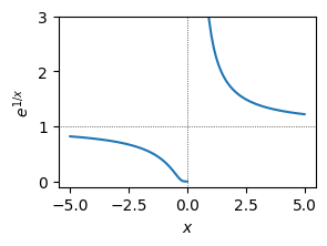
\[\begin{gather*} \Res[f(z=\infty)] = \oint_C f(z) \frac{-z^2\d{w}}{2\pi \I} = -\oint_C \frac{f(1/w)}{w^2} \frac{\d{w}}{2\pi \I} = -\Res\left[\left.\frac{f(1/w)}{w^2}\right|_{w=0}\right]. \end{gather*}\]

_images/7ee582e6a2a747fae0692f47ffbe5a51013f72160eb2ca4d3050bc9c84ca0cb9.png

Example: \(f(z) = e^{1/z}\).

Consider \(f(z) = e^{1/z}\). This is the quintessential example of a function with an essential singularity at \(z=0\). Despite this, the residue still exists, and can be useful for computing contour integrals. To find it, one might try computing the Laurent series, which is straightforward in this case since we know the Taylor series for \(e^{z}\):

\[\begin{gather*} e^{1/z} = \sum_{n=0}^{\infty} \frac{1}{z^{n} n!} = 1 + \frac{1}{z} + \cdots, \qquad \Res[e^{1/z_0}|_{z_0=0}] = 1. \end{gather*}\]

In other cases, however, manipulating products of infinite series might be a pain. Another approach is to note that if the function is meromorphic (analytic everywhere with only isolated singularities), then the sum of all residues is zero:

\[\begin{gather*} \sum_{n} \Res[f(z_n)] = 0. \end{gather*}\]

In this case, we can use the residue at \(z=\infty\):

\[\begin{gather*} \Res[e^{1/z_0}|_{z_0=0}] + \Res[e^{1/z_0}|_{z_0=\infty}] = 0. \end{gather*}\]

Do It! Compute \(\Res[e^{1/z_0}|_{z_0=\infty}]\) and show that this works.

\[\begin{gather*} \Res[e^{1/z_0}|_{z_0=\infty}] = -\Res\left[\left.\frac{e^{w}}{w^2}\right|_{w=0}\right] = -\Res\left[\left.\frac{1+w+\cdots}{w^2}\right|_{w=0}\right]\\ = -\Res\left[\left.\frac{1}{w^2} + \frac{1}{w} + \cdots\right|_{w=0}\right] = -1. \end{gather*}\]

Jordan’s Lemma#

When using contours to compute integrals, it is often important to argue that the contribution from a semi-circular contour vanishes as the radius of that contour is taken to infinity. This is often referred to as Jordan’s Lemma. The Wikipedia formulation is quite useful

Lemma 1 (Jordan’s Lemma)

Let \(f(z)\) be a continuous function in the complex plane \(z \in \mathbb{C}\) with

\[\begin{gather*} f(z) = e^{\I a z}g(z), \qquad a>0, \qquad C_{R} = \{Re^{\I \theta} \mid \theta \in [0, \pi]\}. \end{gather*}\]

Jordan’s Lemma then bounds

\[\begin{gather*} \Abs{\int_{C_{R}} f(z)\d{z}} \leq \frac{\pi}{a}\max_{z\in C_{R}}\abs{g(z)}. \end{gather*}\]

This is especially useful if \(\lim_{R\rightarrow \infty}g(z) = 0\), in which case the contour vanishes. A couple of comments:

This is almost obvious since \(e^{\I a z}\) contains an exponentially decaying piece – the subtlety comes from the regions \(\theta \approx 0\) and \(\theta \approx \pi\) where this exponential piece also vanishes. The lemma proves that one’s intuition remains correct even at these endpoints.
The version in [Hassani, 2013] places an additional constraint that \(R\abs{f(zRe^{\I\theta})} \rightarrow 0\), allowing for the case \(a = 0\), but this excludes the interesting case above. I am not sure why only this from is presented.

Computing Integrals#

The general strategy for computing integrals using contour integration and the residue theorem can be summarized as follows:

Express you original integral as a contour integral.
Try to close the contour in such a way that the added contributions are known, or are expressible in terms of the original integral. JordansLemma is useful here.
Deform the closed contour and compute the integral using the residue theorem.
Remove the additional contributions and solve for the original integral.

# Numerical check.
import math
from scipy.integrate import quad

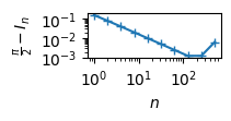
# Quick check.  The integrator has difficulty, but convergence looks good
ns = 2**np.arange(10)
Is = np.array([quad(lambda x: math.sin(x)/x, 0, 2*math.pi * n)[0]
               for n in ns])

fig, ax = plt.subplots(figsize=(2, 1), constrained_layout=True)
ax.loglog(ns, np.pi/2 - Is, '+-')
ax.set(xlabel="$n$", ylabel=r"$\frac{\pi}{2} - I_n$")

# Here we are more careful, using a special purpose integrator
# and pre-computing the first interval so 1/x does not diverge.

I1, I1err = quad(lambda x: math.sin(x)/x, 0, 2*math.pi)
I2, I2err = quad(lambda x: 1/x, 2*math.pi, np.inf, weight='sin', wvar=1.0)
I, Ierr = I1 + I2, I1err + I2err
abs(np.pi/2 - I)

/tmp/ipykernel_3786/3402906312.py:7: IntegrationWarning: The maximum number of subdivisions (50) has been achieved.
  If increasing the limit yields no improvement it is advised to analyze 
  the integrand in order to determine the difficulties.  If the position of a 
  local difficulty can be determined (singularity, discontinuity) one will 
  probably gain from splitting up the interval and calling the integrator 
  on the subranges.  Perhaps a special-purpose integrator should be used.
  Is = np.array([quad(lambda x: math.sin(x)/x, 0, 2*math.pi * n)[0]

3.018052474601518e-11

_images/672878c6d6a1e3b6c17426719136fdd1ac23fab7ea4d60d895ec55514cdc7a62.png

Example: \(I = \int_{0}^{\infty}\tfrac{\sin{x}}{x}\d{x}\).

Let’s start with the example from an early assignment:

\[\begin{gather*} I = \int_{0}^{\infty}\frac{\sin x}{x}\d{x}. \end{gather*}\]

We start by noting that that the integrand is even, so we can compute

\[\begin{gather*} I = \frac{1}{2}\int_{-\infty}^{\infty}\frac{\sin x}{x}\d{x}. \end{gather*}\]

Next, we note that we can express the integral as a contour integral and that the integrand is an analytic function. To close the contour, we consider semi-circle, hoping that this contribution vanishes. Unfortunately, the present integrand does not have nice behaviour at infinity, however, we can split it into two exponentials, each of which vanishes on one of the semicircles:

\[\begin{gather*} I = \frac{1}{2} \int_{-\infty}^{\infty} \left( \frac{e^{\I z}}{2\I z} - \frac{e^{-\I z}}{2\I z}\right) \d{z} \end{gather*}\]

The first term will integrate to zero along an upper semicircle, while the second term will integrate to zero along the lower semicircle. Splitting the integral introduces a pole at \(z=0\) in each term. To deal with this, we must consistently choose to deform the contour either above or below the pole in each term. The result should not depend on which way we choose, as long as we are consistent. Let’s shift it up so that it is contained in the first contour but not the second. This will cause the second contour integral to vanish since there are no poles. Thus, we have

\[\begin{gather*} I = \frac{\pi}{2} \oint \frac{e^{\I z}}{z-\I 0^+}\frac{\d{z}}{2\pi \I} = \frac{\pi}{2} e^{\I (\I 0^+)} = \frac{\pi}{2}. \end{gather*}\]

As a check, if we had shifted the contour down, we would have needed to use the second term which has a minus sign, however, the orientation of the contour also becomes negative, so the two signs cancel and we end up with the same result, as expected.

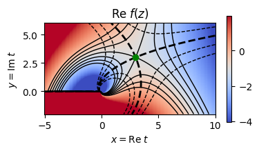
Saddle-point Approximation#

Certain integrals of analytic functions – especially with exponential factors \(e^{f(z)}\) – can be well approximated by deforming the integration contour to include a region where \(\Re f(z)\) is extremal. Since \(f(z)\) is analytic, these extrema must be saddle points since \(u(z) = \Re f(z)\) and \(v(z) = \Im f(z)\) are harmonic. The idea is to approximate the full integral by integrating along the contour of steepest descent, approximating the integrand as a Gaussian along this path:

\[\begin{gather*} \int_{C} e^{f(z)}\d{z} \approx \pm \I e^{f(z_0)}\sqrt{\frac{2\pi}{f''(z_0)}}. \end{gather*}\]

The sign must be chosen to ensure that the saddle is crossed in the appropriate direction consistent with the initial and final points without unnecessary crossings of the “mountain range” over which the saddle provides the cleanest path.

Note

Sometimes the idea of the saddle-point approximation is explained by approximating the integral by the point that maximizes \(u = \Re z\). For contour integrals this does not make much sense since \(u\) is always a saddle point. A better idea is that of stationary phase: by following a contour tangent to the contour of constant \(v(z) = \Im f(z_0)\) that passes through the saddle-point, we can find a contour of constant phase passing through the valley. This contour will give a clean approximation of the integral. Other contours will have larger contributions, but these will cancel due to the rapidly oscillating phase. The contour of constant phase follows the path that descends most rapidly from the saddle point (why?). For this reason, the method is also called the method of steepest descent .

Details.

The orientation of the saddles can be described by the eigenvectors of the corresponding Hessian matrix, and are derived above in section Derivatives: Cauchy-Riemann Conditions with the result that the direction of steepest descent is given by the angles

\[\begin{gather*} \phi_{u} = \frac{\pi-\Phi}{2}, \qquad \phi_{v} = \frac{\pi-\Phi + \tfrac{1}{2}\pi}{2}, \end{gather*}\]

where \(f''(z) = Re^{\I\Phi}\). We integrate along the contour \(C = \{z_0 + se^{\I\phi_u} \mid s \in \mathbb{R}\}\) to find:

\[\begin{align*} f(z) &= f(z_0) + \frac{f''(z_0)}{2!}(z-z_0)^2 + \dots, \\ \int_{C} e^{f(z)}\d{z} &\approx \int_{-\infty}^{\infty}\d{s}\; \exp\left(f(z_0 + se^{\I\phi_u})\right)e^{\I\phi_u}\d{s}\\ &\approx \int_{-\infty}^{\infty}\d{s}\; e^{f(z_0)} \exp\left(\frac{f''(z_0)e^{2\I\phi_u}}{2}s^2\right)e^{\I\phi_u}\d{s}\\ \int_{C} e^{f(z)}\d{z} &\approx \pm \I e^{f(z_0)}\sqrt{\frac{2\pi}{f''(z_0)}} \end{align*}\]

The sign must be chosen to ensure that the saddle is crossed in the appropriate direction consistent with the initial and final points without unnecessary crossings of

Note: this approximation is only valid if the integral is truly dominated by the saddle. To make this clear, most books write

\[\begin{gather*} \int_{C} e^{\alpha h(z)}g(z) \d{z} \end{gather*}\]

where \(\alpha\) is large. This is equivalent to choosing

\[\begin{gather*} f(z) = \alpha h(z) + \ln g(z), \qquad f' = \alpha h' + \frac{g'}{g}, \qquad f'' = \alpha h'' + \frac{gg'' - (g')^2}{g^2}. \end{gather*}\]

_images/b554888b55604cfa68a2ea7c36b3da06ee835c4caf895421a4cc50461afe50b2.png

Example: Sterling’s approximation of \(z! = \Gamma(z+1)\) for large \(\Re z\).

Recall that one can express \(z!\) as

\[\begin{gather*} z! = \int_0^{\infty} t^{z}e^{-t}\d{t} = \int_0^{\infty} e^{z\ln t -t}\d{t}. \end{gather*}\]

Taking \(f(t) = z\ln t - t\), we identify the saddle point \(t_0 = z\) where \(f'(t_0) = 0\):

\[\begin{gather*} f'(t) = \frac{z}{t} - 1,\qquad f''(t) = -\frac{z}{t^2}, \qquad f''(t_0) = -\frac{1}{z}. \end{gather*}\]

The saddle-point approximation gives Stirling’s approximation:

\[\begin{gather*} z! \approx \I z^{z} e^{-z} \sqrt{-2\pi z} = \sqrt{2\pi}\;z^{z+1/2}e^{-z}. \end{gather*}\]

Further Information#

[Needham, 2023] provides an extremely visually pleasing (but lengthy) presentation of complex analysis. Highly recommended if you want to better understand this material. 3Blue1Brown also has some nice videos discussion complex numbers that might help you visualize some of what is going on.

11. Complex Analysis

Contents

11. Complex Analysis#

Analytic Functions#

Multifunctions#

Derivatives: Cauchy-Riemann Conditions#

Conformal Maps and Harmonic Functions#

Infinity#

Möbius Transformations#

Contour Integrals#

Residues#

Laurent Series, Isolated Singularities, and The Residue#

Residue Theorem#

Residue at Infinity#

Jordan’s Lemma#

Computing Integrals#

Saddle-point Approximation#

Further Information#

Analytic Functions #