Class Log - 2025#
These are notes about what we did in class in the Fall 2025 offering of the course.
Mon 1 Dec 2025#
Multi-pole Expansion.
Wed 12 Nov 2025#
Discussed the catenary problem (hanging chain). See Classical Mechanics Notes on Functional Derivatives for complete details.
Also discussed the Legendre-Fenchel transform for a saturating equation of state (see Classical Mechanics Notes on Droplets for details).
Morals:
Look for analogies with Classical Mechanics where you have intuition and rich tools.
Look for symmetries. In this case, the functional was lacking a variable, leading directly to a conservation law.
Mon 10 Nov 2025#
Calculus of Variations. Introduced the catenary problem (hanging chain). See Classical Mechanics Notes on Functional Derivatives for complete details.
Fri 7 Nov#
Central limit theorem. (See Renormalizing Random Walks for details.)
Monte-Carlo integration. Importance sampling. Metropolis algorithm.
Wed 5 Nov#
Bayesian analysis. See Bayesian Analysis and Bayes Factors for details.
Mon 3 Mov 2025#
Probability.
Monte Hall problem.
Bayes theorem.
Meaning of \(\chi^2\) fitting as Bayesian analysis with a flat (uninformed) prior and gaussian errors.
Fri 24 Oct 2025#
Euler-Maclaurin Formula.
Mobius transformation.
Group theory review (Bosons and Fermions).
Wed 22 Oct 2025#
Perturbation theory and Asymptotic Series.
Mittag-Lefler Theorem and \(\zeta(2k)\).
Mon 20 Oct 2025#
Orthogonal Polynomials.
Stone-Weierstrass Theorem.
Gaussian Quadrature.
Bernoulli Numbers.
Fri 17 Oct 2025#
Saddle-point integration and the gamma function \(z! = \int_0^{\infty} t^ze^{-t}\d{t}\).
Wed 15 Oct 2025#
- \[\begin{gather*} \int_0^{\infty} \frac{\sin x}{x}\d{x} \end{gather*}\]
Mon 13 Oct 2025#
Mostly covered stuff in 11. Complex Analysis.
\(\sin(1+\I)\).
\(27^{1/3}\) (all values).
Fundamental theorem of algebra.
Radius of convergence of \(G(x) = 1/(1-x^2)\) and \(H(x) = 1/(1+x^2)\).
Analytic continuation of \(1/(1-x)\) to \(x<-1\).
Fri 10 Oct 2025#
Review of Green’s Functions.
Complex Analysis.
Complex numbers.
\[\begin{gather*} z = x + \I y = r e^{\I\theta}.\\ \frac{1}{1-\I} = \frac{1}{1-\I}\frac{1+\I}{1+\I} = \frac{1+\I}{1-(\I)^2} = \frac{1}{2} + \frac{1}{2}\I.\\ e^{z} = \sum_{n=0}^{\infty} \frac{z^n}{n!}, \qquad \ln(z) = \Log(z) + 2\pi \I n.\\ e^{x+\I y} = e^{x}e^{\I y} = e^{x}(\cos y + \I \sin y).\\ z^w = (e^{\ln(z)})^w = e^{w\ln(z)} = e^{w\Log(z) + 2\pi \I n w}. \end{gather*}\]Multifunctions (Riemann sheets).
\(\ln z\) vs \(\Log(z)\).
\(e^z\) vs \((2.718\dots)^z\).
Clausen’s Paradox: \((e^a)^b = e^{ab} \implies 1 = e^{-2\pi}\) for \(a=2\pi \I\) and \(b=\I\). Resolved by defining \((e^a)^b = e^{b \ln e^a} = e^{b (a + 2\pi \I n)}\). Then \((e^{2\pi \I})^{\I} = e^{\I(2\pi \I + 2\pi \I n)}\), which gives \(1^\I = e^{0}\) for \(n=-1\) as we normally expect.
Wed 8 Oct 2025#
Green’s Functions: For alternative approaches and discussions, see The Pendulum. (Please read.)
Mon 6 Oct 2025#
Midterm Exam 1
Wed 1 Oct 2025#
Review of updated notes on Series and Frobenius’s Method.
General discussion about PDEs: see 9. Partial Differential Equations (PDEs) for details.
Mon 29 Sept 2025#
Discussion of linear algebra, change of bases, and Dirac notation.
Fri 26 Sept 2025#
Discussion of 8. Sturm-Liouville Theory.
Wed 24 Sept 2025#
Discussion of 7. Ordinary Differential Equations (ODEs).
Mon 22 Sept 2025#
Introduction of 7. Ordinary Differential Equations (ODEs).
Fri 19 Sept 2025#
Discussion of 4. Tensors and Manifolds.
Wed 17 Sept 2025#
Discussion of 4. Tensors and Manifolds.
Mon 15 Sept 2025#
Introduction to 4. Tensors and Manifolds.
Fri 12 Sept 2025#
Helmholtz Decomposition.
Question: What does the following matrix do?
\[\begin{gather*} \mat{M} = \begin{pmatrix} 1 & 1\\ 1 & 0 \end{pmatrix}. \end{gather*}\]This corresponds to the coordinate transformation
\[\begin{gather*} x' = x+y, \qquad y' = x \end{gather*}\]Find the eigenvalues and eigenvectors as quickly as possible. Note that \(\mat{M}\) is hermitian.
Matrix factorization.
\(UDV^\dagger\): Singular Value Decomposition (SVD).
Example: Entanglement (Schmidt decomposition)
Did not get to the following:
Hermitian vs self-adjoint. Use finite difference operator as example.
\(L_2\) (see [Hassani, 2013] chapter 7, Thms. 7.2.1-7.2.3
Riesz-Fischer: \(\mathcal{L}^2_{w}(a,b)\) is complete.
All complete inner product spaces with countable bases are isomorphic to \(\mathcal{L}^2_{w}(a,b)\).
Stone-Weierstrass: \(\bigl\{x^n \mid n \in \{0, 1, 2, \dots\}\bigr\}\) forms a basis for \(\mathcal{L}^2_{w}(a,b)\).
Pauli matrices.
Start on Tensors / Differential Geometry.
Metric. Curvilinear coordinates. Jacobian.
Wed 10 Sept 2025#
Angular momentum.
Jacobian.
Differential forms. All vector derivative identities come from
\[\begin{gather*} \int_{V} \d{f} = \int_{\partial V} f\\ \int_{L}f'(x)\d{x} = \int_{\partial L} f(x) = f(L_1) - f(L_0),\\ \int_{V}\vect{\nabla}\cdot \vect{F}\d^{3}x = \int_{\partial V} \vect{F}\cdot\d^2{\vect{A}},\\ \int_{A}(\vect{\nabla}\times\vect{F})\cdot\d^{2}\vect{A} = \int_{\partial A} \vect{F}\cdot\d{\vect{l}}. \end{gather*}\]Operators representing conserved quantities generate the corresponding symmetry transformations:
\[\begin{gather*} e^{\tau\op{H}/\I\hbar}\psi(t) = \psi(t + \tau),\\ e^{\vect{\lambda}\cdot\op{\vect{p}}/\I\hbar}\psi(\vect{x}) = \psi(\vect{x} - \vect{\lambda}),\\ e^{\vect{\theta}\cdot\op{\vect{L}}/\I\hbar}\psi(\vect{x}) = \psi(\mat{R}_\vect{\theta}^{-1}\vect{x}), \qquad \mat{R}_{\vect{\theta}} = e^{\mat{\vect{\theta}\times}}. \end{gather*}\]
Mon 8 Sept 2025#
Discussion of vectors as curves, and some of the meaning of things like div, grad, and curl. (Incomplete)
Types of linear transforms: Scaling, Rotation, Shears.
Hermitian matrices have a complete orthonormal basis.
Completeness
\[\begin{gather*} \mat{1} = \sum_{n}\ket{n}\bra{n} = \int \ket{x}\bra{x}\d{x} = \int \ket{k}\bra{k}\frac{\d{k}}{2\pi}, \qquad \braket{x|k} = e^{\I k x}, \end{gather*}\](using my normalizations).
Show that this gives the Fourier transform:
\[\begin{gather*} \psi_k = \braket{k|\psi} = \braket{k|\mat{1}|\psi} = \int\braket{k|x}\braket{x|\psi}\d{x} = \int e^{-\I k x}\psi(x)\d{x} \end{gather*}\]Jordan Normal Form
SVD
Question: What does the following matrix do?
\[\begin{gather*} \mat{M} = \begin{pmatrix} 1 & 1\\ 1 & 0 \end{pmatrix}. \end{gather*}\]This corresponds to the coordinate transformation
\[\begin{gather*} x' = x+y, \qquad y' = x \end{gather*}\]
Fri 5 Sept 2025#
Rotation matrices.
Linear approximations.
Quick overview of Groups and Lie Algebras.
Wed 3 Sept 2025#
Levi-Civita symbol.
Vectors and matrices, especially projection operators.
Fri 29 Aug 2025#
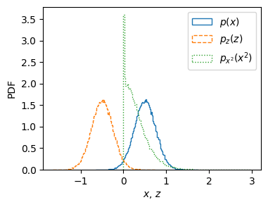
Problem for the day (from Wed): Given a random variable \(x\) with PDF \(p(x)\), what is the PDF \(p_z(z)\) for \(z = f(x)\)?
For example, if \(f(x) = x-a\), then you should find \(p_z(z) = p(z+a)\).
plan
Gram-Schmidt:
Mentioned that functions are vectors.
\[\begin{gather*} \braket{f|g} = \int \d{x} f^*(x) g(x) \textcolor{green}{w(x)}. \end{gather*}\]Unifies fourier, orthogonal polynomials, many special functions, etc.
Some power series:
\[\begin{gather*} \ln(1-x) = x + \frac{x^2}{2} + \cdots + \frac{x^{n}}{n} + \cdots.\\ \end{gather*}\]Dirac delta function. Distribution.
Finite differences.
Wed 27 Aug 2025#
Discussion of adding errors in quadrature: I.e., exactly what it means to say that if \(x = \bar{x} \pm \sigma_x\) and \(y = \bar{y} \pm \sigma_y\), then
Demonstrate that if \(x\) and \(y\) are independent random variables with PDFs \(p_x(x)\) and \(p_y(y)\), then \(z = x+y\) has PDF
I.e., \(p_z\) is the convolution of \(p_x\) and \(p_y\).
Mentioned (no derivation) the following logic:
\(x = \bar{x} \pm \sigma_x\) means \(x \sim \mathcal{N}_{\mu=\bar{x}, \sigma=\sigma_x}\) is normally distributed with mean \(\bar{x}\) and standard deviation \(\sigma_x^2\).
The PDF \(p_x(x)\) is thus a gaussian with variance \(\sigma_x^2\).
The Fourier transform of this is also a gaussian with variance \(1/\sigma_x^2\). (This is a manifestation of the uncertainty principal.)
The convolution theorem tells us that the Fourier transform of \(p_z = p_x*p_y\) is just the project of the Fourier transforms:
\[\begin{gather*} \mathcal{F}(p_z) = \mathcal{F}(p_x)\mathcal{F}(p_y). \end{gather*}\]The PDF \(p_z(z)\) is thus a gaussian with covariance \(\sigma_z^2 = \sigma_x^2 + \sigma_y^2\): i.e. the covariances add. This follows directly from the fact that
\[\begin{gather*} \mathcal{F}(p_{x}) \propto e^{-k^2 \sigma_{x}^2/2}, \qquad \mathcal{F}(p_{z}) = \mathcal{F}(p_{x})\mathcal{F}(p_{y}) \propto e^{-k^2 \sigma_{x}^2/2} e^{-k^2 \sigma_{x}^2/2} = e^{-k^2 (\sigma_{x}^2 + \sigma_y^2)/2}. \end{gather*}\]
Mentioned that even for non-Gaussian variables, the covariances add \(\sigma_z^2 = \sigma_x^2 + \sigma_y^2\), but that the shape of the distribution might change.
Mentioned that this also holds for linear transformations \(z = ax + by +c\). Since every “nice” function is approximately linear if you zoom in far enough, once you have small enough errors you can use the quadrature rule. But don’t forget the limitations:
The errors are small enough that the function is linear over the range of errors.
The errors are independent.
The errors are gaussian. *(Not strictly needed, but implicit in the notation \(\mu\pm \sigma\).
Mentioned the Weierstrass M-test and Abel’s test, discussed Cauchy convergence, and how limits might not exist, e.g., the real numbers (with cardinality \(\aleph_1\): i.e. uncountable) can be formed as the collection of convergent Cauchy sequences of rational numbers (which have cardinality \(\aleph_0\): i.e. countable).
Mon 25 Aug 2025#
Inner product spaces: Some confusion. (E.g. Notion of angle in complex spaces?)
Discussion of matrices and vectors. \((\mat{A}\mat{B})^\dagger = \mat{B}^\dagger\mat{A}^\dagger\).
Index notation to make sure:
\[\begin{gather*} [(\mat{A}\mat{B})^\dagger]_{ik} = A_{kj}^*B_{ji}^* = B_{ji}^*A_{kj}^* = [\mat{B}^\dagger]_{ij}[\mat{A}^\dagger]_{jk} = [\mat{B}^\dagger\mat{A}^\dagger]_{ik}. \end{gather*}\]
Fri 22 Aug 2025#
Feynman’s differentiation trick.
Series, convergence.
Review of better method of series convergence: integral test + generalized ratio test. See notes in 1. Mathematical Preliminaries.
Alternating series that are not absolutely convergent can sum to anything.
Mentioned that functions are vectors.
\[\begin{gather*} \braket{f|g} = \int \d{x} f^*(x) g(x) \textcolor{green}{w(x)}. \end{gather*}\]Unifies fourier, orthogonal polynomials, many special functions, etc.
Wed 20 Aug 2025#
Introductions.
Technical problem: Are the following limits convergent or divergent?
\[\begin{gather*} u_{n} = \frac{1}{n^s (\ln n)^t}, \qquad \lim_{N\rightarrow\infty}\int^{N} u_n\d{n}, \qquad \lim_{n\rightarrow\infty} \frac{u{n+1}}{u_{n}}. \end{gather*}\]Quick review of linear algebra.
Need review of Inner Product Spaces, SVD, etc.
Did the matrix exponential:
\[\begin{gather*} e^{\mat{M}} = \lim_{N\rightarrow \infty} \sum_{n=0}^{N} \frac{\mat{M}^{n}}{n!} \end{gather*}\]Discussed how to learn: how I learn.
Quick review of Syllabus, reading assignment.