18. More Special Functions

18. More Special Functions#

Here we consider some functions not included in [Arfken et al., 2013].

Airy Function#

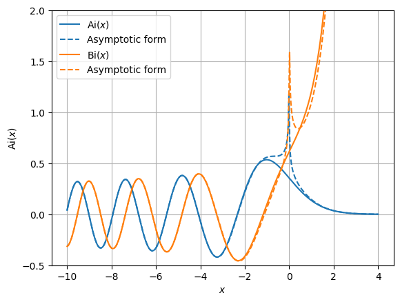
The Airy functions $\Ai(x)$ and $\Bi(x)$ for real arguments $x$ can be defined as

\[\begin{align*} \Ai(x) &= \frac{1}{\pi}\int_0^{\infty}\cos\left(xt + \frac{t^3}{3}\right)\d{t}\,,\\ \Bi(x) &= \frac{1}{\pi}\int_0^{\infty}\left[ \sin\left(xt + \frac{t^3}{3}\right) -\exp\left(xt - \frac{t^3}{3}\right) \right]\d{t}\,.\\ \end{align*}\]

Do It! Show that these converge.

Hint: Consider this as an alternating series of half-periods of decreasing width. Show that the magnitude of each term decreases, hence the series converges (conditionally). This is an application of Dirichlet’s test.

This function arises from the quantum mechanics of a particle falling in a constant gravitational field:

\[\begin{gather*} \op{H} = \frac{\op{p}^2}{2m} + mg\op{z}. \end{gather*}\]

In appropriate units, the solution can be expressed as

\[\begin{gather*} -\psi''(z) + (z-E)\psi(z) = 0, \qquad \psi(z) = a\Ai(z-E) + b\Bi(z-E), \end{gather*}\]

where the Airy functions $y=\Ai(x)$ and $y=\Bi(x)$ above, which satisfy:

\[\begin{gather*} y'' = xy. \end{gather*}\]

Do It! Find the appropriate units where this works.

Dimensionally,

\[\begin{gather*} [\hbar] = \frac{MD^2}{T}, \qquad [m] = M, \qquad [g] = \frac{D}{T^2}, \end{gather*}\]

so we can choose units $\hbar = 2m = g/2 = 1$ so that

\[\begin{gather*} 1 = \underbrace{2m}_{\text{mass}} = \overbrace{\underbrace{\left(\frac{\hbar^2}{2m^2g}\right)^{1/3}}_{\text{length}}}^{\xi} = \underbrace{\left(\frac{2\hbar}{mg^2}\right)^{1/3}}_{\text{time}} = \underbrace{\left(\frac{\hbar^2 mg^2}{2}\right)^{1/3}}_{\text{energy}} = \underbrace{\left(\hbar 2m^2g\right)^{1/3}}_{\text{momentum}}. \end{gather*}\]

In these units, the time-independent Schrödinger equation has the form

\[\begin{gather*} -\psi''(z) + (z-E)\psi(z) = 0, \end{gather*}\]

as stated.

Do It! Solve $y'' - xy = 0$.

Hint: try to find a solution of the form

\[\begin{gather*} y(x) = \int_{C} e^{xz}v(z)\d{z} \end{gather*}\]

over some appropriate contour $C$.

Solution

The trick is to notice that

\[\begin{gather*} xy(x) = \int_{C} xe^{xz}v(z)\d{z} = \int_{C} \diff{e^{xz}}{z} v(z)\d{z} = - \int_{C} e^{xz}v'(z) \d{z} \end{gather*}\]

if we choose a contour $C$ where the boundary term vanishes. Then,

\[\begin{gather*} y'(x) = \int_{C} ze^{xz}v(z)\d{z}, \qquad y''(x) = \int_{C} z^2e^{xz}v(z)\d{z}, \end{gather*}\]

hence, we must find $v(z)$ such that

\[\begin{gather*} y''(x) - xy(x) = \int_{C} \bigl(z^2v(z) + v'(z)\bigr)e^{xz}v(z)\d{z} = 0. \end{gather*}\]

A viable solution is to choose $v(z)$ such that $z^2v(z) + v'(z) = 0$. This is separable

\[\begin{gather*} z^2 \d{z} = - \frac{\d{v}}{v} = -\d{\ln v},\\ -\ln v = \frac{z^3}{3},\\ v(z) = e^{-z^3/3}. \end{gather*}\]

Hence, up to an overall factor (not specified by the differential equation),

\[\begin{gather*} y(x) = \int_{C} e^{xz-z^3/3}\d{z}. \end{gather*}\]

To ensure that the boundary term vanishes, we can choose $C$ so that $v(z) \rightarrow 0$ at the boundaries – i.e., going to infinity in regions where $\Re z^3$ is positive. One way to do this is as the contour integral

\[\begin{gather*} \Ai(x) = \int_{-\I\infty - 0^+}^{\I\infty - 0^+} e^{xz - z^3/3}\frac{\d{z}}{2\pi \I} \end{gather*}\]

which turns out to be the Airy function as defined above:

\[\begin{gather*} z = \I t, \qquad \d{z} = \I \d{t}, \qquad z^3 = -\I t^3,\\ \Ai(x) = \int_{-\infty + \I 0^+}^{\infty + \I 0^+} e^{\I(x t + t^3/3)}\frac{\d{t}}{2\pi}\\ = \frac{1}{2\pi}\int_{-\infty}^{\infty} \cos\left(\frac{t^3}{3} + xt\right) \d{t}\\ = \frac{1}{\pi}\int_{0}^{\infty} \cos\left(\frac{t^3}{3} + xt\right) \d{t}. \end{gather*}\]

Do It! Show that $\Ai(x)$ as defined above satisfies this equation.

\[\begin{align*} \Ai'(x) &= \frac{1}{\pi}\int_0^{\infty} (-t)\sin\left(\frac{t^3}{3} + xt\right)\d{t},\\ \Ai''(x) &= \frac{1}{\pi}\int_0^{\infty} (-t^2)\cos\left(\frac{t^3}{3} + xt\right)\d{t}. \end{align*}\]

Noting that

\[\begin{gather*} t^2 = \diff{}{t}\left(\frac{t^3}{3} + xt\right) - x, \end{gather*}\]

we have

\[\begin{gather*} \Ai''(x)= -\frac{1}{\pi}\int_0^{\infty} \diff{}{t}\left(\frac{t^3}{3} + xt\right) \cos\left(\frac{t^3}{3} + xt\right)\d{t} + x\underbrace{\frac{1}{\pi}\int_0^{\infty} \cos\left(\frac{t^3}{3} + xt\right)\d{t}} _{x\Ai(x)}. \end{gather*}\]

It remains to show that the other piece is zero, which we can do by changing variables to $\theta = t^3/3 + xt$:

\[\begin{gather*} \int_0^{\infty} \diff{}{t}\left(\frac{t^3}{3} + xt\right) \cos\left(\frac{t^3}{3} + xt\right)\d{t} = \int_0^{\infty} \diff{\theta}{t}\cos\theta\d{t} = \int_0^{\infty} \cos\theta\d{\theta} = \left.\sin\theta\right|^{\infty}_{0}. \end{gather*}\]

We can ensure this vanishes by keeping a slight imaginary part to $t$.

Asymptotic Properties#

The asymptotic properties of $\Ai(x)$ can be found by using the Saddle-point Approximation from the representation given in the solution above

\[\begin{gather*} \Ai(x) = \int_{-\I\infty - 0^+}^{\I\infty - 0^+} e^{xz - z^3/3}\frac{\d{z}}{2\pi \I} = \frac{1}{2\pi \I}\int_{C}f^{f(z)}\d{z} \end{gather*}\]

where $f(z) = xz - z^3/3$. Notice that the contour integral is along the imaginary axis, so if $\abs{x} \gg 1$ is large, then the phase $xz$ oscillates rapidly, and the integral will be dominated by stationary regions where $f'(z) \approx 0$.

\[\begin{gather*} f'(z) = x - z^2\,, \qquad f''(z) = -2z\,, \\ \qquad f'(z_0) = 0\,, \qquad z_0 = \pm \sqrt{x}\,,\\ f(z_0) = \pm \frac{2}{3}x^{2/3} = \pm \xi\,\qquad f''(z_0) = \mp 2\sqrt{x}. \end{gather*}\]

To simplify some formula, we follow [Vallée and Soares, 2010] and define $\xi = \tfrac{2}{3}x^{2/3}$.

If $x>0$, then the contour naturally goes through the negative root $z_0 = -\sqrt{x}$, and we have

\[\begin{align*} \Ai(x) \approx \frac{\I}{2\pi \I} e^{f(z_0)}\sqrt{\frac{2\pi}{f''(z_0)}} &= \frac{1}{2\pi^{1/2}x^{1/4}}e^{-2x^{3/2}/3}\,, & x&\gg 1\,,\\ \Bi(x) &\approx \frac{1}{\pi^{1/2}x^{1/4}}e^{2x^{3/2}/3}\,, & x&\gg 1\,. \end{align*}\]

I have not derive the form for $\Bi(x)$ yet, but this is correct. If $x<0$, then the two roots move to the imaginary axis, and we should consider the sum of both contributions $z_0 = \pm \I \sqrt{-x}$:

\[\begin{align*} \Ai(x) \approx \frac{e^{2\I(-x)^{3/2}/3}}{\sqrt{\I\pi}(-x)^{1/4}} - \frac{e^{-2\I(-x)^{3/2}/3}}{\sqrt{-\I\pi}(-x)^{1/4}} &= \frac{2}{\pi^{1/2}(-x)^{1/4}}\sin\left(\frac{2(-x)^{3/2}}{3} + \frac{\pi}{4}\right) \,, & x &\ll -1\,,\\ \Bi(x) &\approx \frac{2}{\pi^{1/2}(-x)^{1/4}}\cos\left(\frac{2(-x)^{3/2}}{3} + \frac{\pi}{4}\right) \,,& x &\ll -1\,. \end{align*}\]

Note that the $\pi/4$ phase shift comes from the factor of $\sqrt{\I} = e^{\pm \I \pi / 4}$. There is some ambiguity in the signs of the various pieces that need to be checked carefully. The form given is correct, and with the phase choice, shows the simple relationship between $\Ai(x)$ and $\Bi(x)$ We verify this form numerically below:

_images/78d55c2f0ae21d4e93d5bc9cc2f6537c7b3f1a2ce2b0e1835e87728c6781ba16.png

Complete Expansion (incomplete and incorrect)

A complete expansion can be obtained by changing variables:

\[\begin{gather*} \frac{z^3}{3} - xz = z\left(\frac{z^2}{3} - x) = \frac{-2x^{3/2}}{3} - v^2\\ (z^2 - x)\d{z} = -2v\d{v}. \end{gather*}\]

$z = \sqrt{x} + \I w$,

\[\begin{gather*} \Ai(x) = \int_{-\I\infty - 0^+}^{\I\infty - 0^+} e^{z^3/3 - xz}\frac{\d{z}}{2\pi \I} = \int_{-\infty + \I 0^+}^{\infty + \I 0^+} e^{z^3/3 - xz}\frac{\d{w}}{2\pi} \end{gather*}\]

A complete expansion can be obtained by changing variables $z = \sqrt{x} + \I \sqrt{w\sqrt{x}}$, $

\[\begin{gather*} (z - \sqrt{x})^2 = z^2 + x - 2z\sqrt{z} = - w\sqrt{x}\\ \frac{z^3}{3} - zx = \left(\frac{z^2}{3}-x\right)z \\ = \frac{\left(-2x - wx^{1/2} + 2\I w^{1/2}x^{3/4}\right)(x^{1/2} + \I w^{1/2}x^{1/4})}{3}\\ \frac{-2x^{3/2} - wx + 2\I w^{1/2}x^{5/4} -2\I x^{4/4}w^{1/2} - \I w^{3/2}x^{3/4} - 2wx }{3}\\ = \frac{-2x^{3/2}}{3} + \frac{- 3wx - \I w^{3/2}x^{3/4}}{3}\\ \d{z} = \frac{\I x^{1/4}}{2w^{1/2}}\d{w}\\ \Ai(x) = \int_{-\I\infty - 0^+}^{\I\infty - 0^+} e^{z^3/3 - xz}\frac{\d{z}}{2\pi \I} = \int_{-\I\infty - 0^+}^{\I\infty - 0^+} e^{z^3/3 - xz}\frac{\d{z}}{2\pi \I} \frac{\I x^{1/4}}{2w^{1/2}} \end{gather*}\]

Green’s Function#

We can also find the Green’s function [Vallée and Soares, 2010]:

\[\begin{gather*} G(z,z') = -\pi \begin{cases} \Ai(z')\bigl(\Bi(z) + \I\Ai(z)\bigr) & z \leq z',\\ \Ai(z)\bigl(\Bi(z') + \I\Ai(z')\bigr) & z \geq z' \end{cases}, \\ \left(\pdiff[2]{}{z} - z\right)G(z, z') = \delta(z-z') \end{gather*}\]

This gives, for example, the steady state solution $G(z,0)$ for a continuous atom laser with particles continually being injected at $z'=0$.

For $z<0$, the qualitative form can be deduced from the WKB approximation:

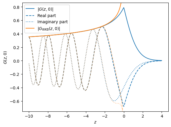
\[\begin{gather*} \psi_{\mathrm{WKB}}(z) \propto \frac{1}{\sqrt{p(z)}}e^{S(z)/\I\hbar}, \\ z(t) = - \frac{gt^2}{2}, \qquad p(z) = -mgt = -m\sqrt{-2gz}\\ S(z) = \int_0^{t}\left(\frac{p^2}{2m} - mgz(t)\right)\d{t} = \frac{-mg^2t^3}{3} = -\hbar \frac{2}{3}\sqrt{\frac{-z^3}{\xi^3}},\\ \psi_{\mathrm{WKB}}(z) \propto \frac{1}{\abs{z}^{1/4}} \exp\left(\frac{2\I}{3}\sqrt{\frac{-z^3}{\xi^3}}\right) \end{gather*}\]

_images/d7be258fc7abfc905caa032086f9cbd9a2e5072a8e8a1504d7552d0332dbd4b6.png

Once properly normalized, this gives a very good approximation except very close to the injection site which is a classical turning point and the WKB approximation breaks down.

Atom Laser

An atom laser can be produced by “out-coupling” a trapped state (the source) to the falling state with the following two-component Hamiltonian

\[\begin{gather*} \op{H} = \begin{pmatrix} \frac{\op{p}_z^2}{2m} + mg\op{z} & \Omega e^{\I\omega t}\\ \Omega e^{-\I\omega t} & \frac{\op{p}_z^2}{2m} + V(\op{z}) \end{pmatrix}. \end{gather*}\]

The idea of an atom laser is that a large reservoir of the lower component is held in the trapping potential $V(z)$. The off-diagonal coupling converts this lower component to the upper component, which falls in the gravitational field. If the off-diagonal coupling is small, the one can treat the trapped component as a constant, and we have the following coupled equation (essentially neglecting the lower-left block):

\[\begin{align*} \I\hbar \ket{\dot{\psi}_a(t)} &= \left(\frac{\op{p}_z^2}{2m} + mg\op{z}\right)\ket{\psi_a(t)} + \Omega e^{\I\omega t}\ket{\psi_b(t)}\\ \I\hbar \ket{\dot{\psi}_b(t)} &= \left(\frac{\op{p}_z^2}{2m} + V(\op{z}) - E_b\right)\ket{\psi_b(t)}. \end{align*}\]

After some time, the states become quasi-stationary, and we can write:

\[\begin{gather*} \ket{\psi_b(t)} = \ket{\psi_b}e^{-\I E_b t/\hbar}, \qquad \ket{\psi_a(t)} = \ket{\psi_a}e^{\I (\hbar \omega - E_b) t /\hbar},\\ \begin{aligned} \left(\frac{\op{p}_z^2}{2m} + mg\op{z} - \I\hbar \partial_t\right)\ket{\psi_a(t)} &= - \Omega e^{\I(\hbar \omega - E_b)t/\hbar}\ket{\psi_b},\\ \left(\frac{\op{p}_z^2}{2m} + V(\op{z}) - E_b\right)\ket{\psi_b} &= 0,\\ \left(\frac{\op{p}_z^2}{2m} + mg\op{z} + \hbar \omega - E_b\right)\ket{\psi_a} &= -\Omega \ket{\psi_b},\\ \left(\frac{\op{p}_z^2}{2m} + mg(\op{z} + z_0)\right)\ket{\psi_a} &= -\Omega \ket{\psi_b},\\ \end{aligned} \end{gather*}\]

The bottom equation was simplified by setting $mgz_0 = \hbar \omega - E_b$, which we can redefine as the zero of our coordinate system $z \rightarrow z - z_0$. Doing this, and switching to our natural units, we have:

\[\begin{gather*} \left(\pdiff[2]{}{z} - z\right)\psi_a(z-z_0) = \Omega \psi_b(z-z_0) =\\ = \Omega\int\d{z'}\;\psi_b(z'-z_0)\delta(z-z'). \end{gather*}\]

Hence, our solution can be expressed in terms of the Green’s function:

\[\begin{gather*} \psi_a(z-z_0) = \Omega \int\d{z'}\; G(z,z') \psi_b(z' - z_0)\\ \psi_a(z) = \Omega \int\d{z'}\; G(z+z_0,z'+z_0)\psi_b(z'). \end{gather*}\]

The Green’s function is quite sharply peaked about $\abs{z-z'} \lesssim 2$, so the laser out-couples atoms from a fairly narrow region about

\[\begin{gather*} \abs{z - z_0} \lesssim \sqrt[3]{\frac{4\hbar^2}{m^2g}}, \end{gather*}\]

the location of which can be tuned by adjust the drive frequency $\omega$.

Atom Interferometry#

An application of the atom laser is to image differential potentials (see e.g. .) In this application, we have two streams of particles, which experience slightly different potentials

\[\begin{gather*} V_{a,b}(z) = V_0(z) \pm V(z). \end{gather*}\]

The corresponding actions are (see eg:FallingParticles):

\[\begin{gather*} S_{a,b}(z;z_0; E) = -Et \pm \int_{z_0}^{z} p_{a,b}(z)\d{z}, \\ p_{a,b}(z) = \sqrt{2m(E-V_{a,b}(z))}. \end{gather*}\]

For a falling particle with, we can set $z_0 = 0$, $E=0$, and $V_0(z) = mgz$. An interferometer allows us to recover the relative phase difference, so by differentiating, we can directly extract $V(z)$:

\[\begin{align*} S_a'(z) - S_b'(z) &= -p_a(z) + p_b(z) \\ &= \sqrt{-2m^2 gz + 2mV(z)} - \sqrt{-2m^2 gz - 2mV(z)}. \end{align*}\]

If $V(z)$ is small, we can expand:

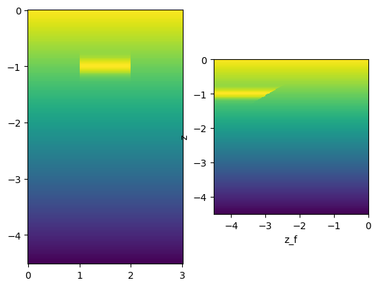
\[\begin{gather*} V(z) \approx \sqrt{\frac{-gz}{2}}\Bigl(S_a'(z) - S_b'(z)\Bigr) \end{gather*}\]

The experiment is slightly more complicated in that the differential potential is pulsed on for a short period of time:

\[\begin{gather*} V_{a,b}(z, t) = V_0(z) \pm V(z)\mathbf{1}_{[t_1, t_2]}(t). \end{gather*}\]

To deal with this, we define the trajectory $z(t, z_f)$ for the particle ending up at $z(t_f, z_f) = z_f$ at imaging time $t_f$. We can then use the same formalism with the potential, but now with a potential that depends on $z_f$. Assuming again that $z_0=0$, $E=0$, and that the particle is falling, we have

\[\begin{gather*} V_{a, b}(z; z_f) = V_0(z) \pm V(z)\mathbf{1}_{[z(t_1;z_f),z(t_2;z_f)]}(z),\\ S_{a,b}(z_f) = -\int_{z_0}^{z_f} p_{a,b}(z;z_f)\d{z}, \\ \begin{aligned} p_{a, b}(z;z_f) &= \sqrt{-2mV_{a,b}(z;z_f)}\\ &\approx \sqrt{-2m V_0(z)} \pm \frac{mV(z)}{\sqrt{-2mV_0(z)}}\mathbf{1}_{[z(t_1;z_f),z(t_2;z_f)]}(z) \end{aligned} \end{gather*}\]

The derivative is slightly more complicated now because of the addition $z_f$ dependence in the momentum:

\[\begin{gather*} \pdiff{V_{a,b}(z;z_f)}{z_f} = \pm V(z)[\delta\bigl(z-z(t_2, z_f)\bigr) - \delta\bigl(z-z(t_1;z_f)\bigr)],\\ \begin{aligned} \pdiff{p_{a,b}(z;z_f)}{z_f} &= \sqrt{\frac{-m}{2V_{a,b}(z;z_f)}}\pdiff{V_{a,b}(z;z_f)}{z_f}\\ &= \frac{m}{p_{a,b}(z;z_f)}\pdiff{V_{a,b}(z;z_f)}{z_f}, \end{aligned} \end{gather*}\]

This gives:

\[\begin{gather*} S_{a, b}'(z_f) = -p_{a,b}(z_f;z_f) -\int_{z_0}^{z_f} \pdiff{p_{a,b}(z;z_f)}{z_f}\d{z},\\ = -p_{a,b}(z_f;z_f) \mp\left. \frac{m V(z)}{p_{a,b}(z;z_f)}\right|_{z=z_2=z(t_2;z_f)}^{z=z_1=z(t_1;z_f)}. \end{gather*}\]

In a typical experiment, the differential potential is turned off at the imaging time, so $p_{a}(z_f;z_f) = p_{b}(z_f;z_f)$, so the first term – which gives the dominant contribution above – vanishes, leaving the following difference in the action:

\[\begin{align*} S_a'(z_f) - S_b'(z_f) &= \left. -m V(z)\left( \frac{1}{p_{b}(z;z_f)} + \frac{1}{p_{a}(z;z_f)} \right) \right|_{z=z_2=z(t_2;z_f)}^{z=z_1=z(t_1;z_f)}\\ &\approx \left. \frac{-2mV(z)}{\sqrt{-2mV_0(z)}} \right|_{z=z_2=z(t_2;z_f)}^{z=z_1=z(t_1;z_f)}. \end{align*}\]

t_1 = 1.0
t_2 = 2.0
t_f = 3.0
g = 1.0
m = 1.0
z_f = -g*t_f**2/2

z_V = -1.0
sigma = 0.1
dV = 1.0

@np.vectorize
def V(z, t):
    return m*g*z + dV * np.exp(-(z-z_V)**2/2/sigma**2)*np.where(t_1 < t < t_2, 1, 0)

@np.vectorize
def Vzf(z, z_f):
    # How long the particle takes to get to z
    dt = np.sqrt(-2*z/g)
    # How long the particle takes to get to z_f dtf = (t_f-t_0)
    dtf = np.sqrt(-2*z_f/g)
    t_0 = t_f - dtf
    t = t_0 + dt
    return V(z=z, t=t)

t, z = np.meshgrid(np.linspace(0, t_f, 200), 
                   np.linspace(z_f, 0, 201), 
                   indexing='ij', sparse=True)
fig, axs = plt.subplots(1, 2)
ax = axs[0]
ax.pcolormesh(t.ravel(), z.ravel(), V(z, t).T, shading='auto')

ax = axs[1]
zf = z.T
ax.pcolormesh(zf.ravel(), z.ravel(), Vzf(z, zf).T, shading='auto')
ax.set(xlabel="z_f", ylabel="z", aspect=1);

_images/7737b7e26a83e5298a6867422f90b34d9cc11a38def65522e6b2e61262b94b8b.png

(Old Stuff)#

from ipywidgets import interact
from scipy.special import airy

hbar = 1
m = 0.5
g = 2.0
Omega = 0.1

sigma = 1.0

z = np.linspace(-100, 2, 500)
Ai0, dAi0, Bi0, dBi0 = airy(0)
Aiz, dAiz, Biz, dBiz = airy(z)

def G(x, xx=0):
    Aix, dAix, Bix, dBix = airy(x)
    Ai0, dAi0, Bi0, dBi0 = airy(xx)
    return (
        - np.pi * np.where(x < xx, Ai0 * (Bix + 1j * Aix), Aix * (Bi0 + 1j * Ai0))
    )

@interact(sigma=(0.01, 10.0))
def go(sigma=1.0):
    def psi_b(z):
        return np.exp(-(z/sigma)**2/2)
    
    zz = np.linspace(-4*sigma, 4*sigma, 200)
    psi_a = Omega*G(z[:, None], zz[None, :]) @ psi_b(zz)
    n_a = abs(psi_a)**2
    n_b = abs(psi_b(z))**2
    fig, ax = plt.subplots()
    ax.plot(z, n_a, 'C0', label='$n_a(z)$')
    ax.twinx()plot(z, n_b, 'C1', label='$n_b(z)$')
    ax.set(xlabel='$z$', ylabel="$n_a$")
    ax.grid(True)
    ax.legend();

  Cell In[5], line 33
    ax.twinx()plot(z, n_b, 'C1', label='$n_b(z)$')
              ^
SyntaxError: invalid syntax

def psi_b(z):
    return np.exp(-(z/sigma)**2/2)

zz = np.linspace(-2*sigma, 2*sigma, 100)
psi_a = G(z[:, None], zz[None, :]) @ psi_b(zz[None, :])

plt.plot(z, abs(G(z, 2.0))**2)

---------------------------------------------------------------------------
ValueError                                Traceback (most recent call last)
Cell In[6], line 5
      2     return np.exp(-(z/sigma)**2/2)
      4 zz = np.linspace(-2*sigma, 2*sigma, 100)
----> 5 psi_a = G(z[:, None], zz[None, :]) @ psi_b(zz[None, :])
      7 plt.plot(z, abs(G(z, 2.0))**2)

Cell In[3], line 12, in G(x, y)
      9 Aix, dAix, Bix, dBix = airy(x)
     10 Aiy, dAiy, Biy, dBiy = airy(y)
     11 return (
---> 12     - np.pi * np.where(x < y, Aiy * (Bix + 1j * Aix), Aix * (Biy + 1j * Aiy))
     13 )

ValueError: operands could not be broadcast together with shapes (1,1,201) (1,100) 

Gz = G(z)

@interact(ar=(-2,2,0.001), ai=(-2,2,0.001))
def go(ar=-np.sqrt(3)/4/np.pi/Ai0**2, ai=1/4/np.pi/Ai0**2):
    a = ar + ai*1j
    alpha = 1/a/Ai0 + np.pi * (np.sqrt(3) + 1j)*Ai0
    psi = Gz + alpha * Aiz
    n = abs(psi)**2
    n_wkb = 1/m/np.sqrt(-2*g*z)
    n_wkb *= n[0]/n_wkb[0]
    j = (-1j * hbar * np.gradient(psi, z) * psi.conj()).real
    fig, ax = plt.subplots()
    ax.plot(z, n, label='$n(z)$')
    ax.plot(z, j, ls='--', label='$j(z)=n(z)v(z)$')
    ylim = ax.get_ylim()
    ax.plot(z, n_wkb, ls=':', label='$n_{WKB}(z)$')
    ax.set(xlabel='$z$', ylabel="$n$, $j$", ylim=ylim)
    ax.grid(True)
    ax.legend();

---------------------------------------------------------------------------
NameError                                 Traceback (most recent call last)
Cell In[7], line 3
      1 Gz = G(z)
----> 3 @interact(ar=(-2,2,0.001), ai=(-2,2,0.001))
      4 def go(ar=-np.sqrt(3)/4/np.pi/Ai0**2, ai=1/4/np.pi/Ai0**2):
      5     a = ar + ai*1j
      6     alpha = 1/a/Ai0 + np.pi * (np.sqrt(3) + 1j)*Ai0

NameError: name 'interact' is not defined

Old Discussion: Potential Source

Note that we can add to $G(z, z')$ any solution of the homogeneous equation, so we can write:

\[\begin{gather*} \psi(z) = G(z, 0) + \alpha \Ai(z),\\ \Bigl(-\pdiff[2]{}{z} + z + \overbrace{\frac{1}{\psi(0)}}^{a}\delta(z)\Bigr)\psi(z) = 0. \end{gather*}\]

This is the steady state solution with $E=0$ to the time-independent Schrödinger equation with a delta-function potential of strength $a = 1/\psi(0)$. If this has an imaginary part, then we have a particle source of sink. Inverting, we have:

\[\begin{gather*} \Bi(0) = \sqrt{3}\Ai(0) = \frac{\sqrt{3}}{3^{2/3}\Gamma(\tfrac{2}{3})},\\ G(0,0) = -\pi\left(\Ai(0)\Bi(0) + \I \Ai^2(0)\right) = -\pi\left(\sqrt{3} + \I\right)\Ai^2(0),\\ a^{-1} = \psi(0) = -\pi\Bigl(\sqrt{3} + \I\Bigr)\Ai^2(0) + \alpha \Ai(0),\\ \alpha = \frac{1}{a\Ai(0)} + \pi\Bigl(\sqrt{3} + \I\Bigr)\Ai(0). \end{gather*}\]

In the region $z < 0$ the solution will have the form:

\[\begin{gather*} \psi(z<0) = -\pi\Ai(0)\left(\Bi(z) + \I \Ai(z)\right) + \alpha \Ai(z),\\ = -\pi\Ai(0)\left( \Bi(z) - \Bigl(\sqrt{3} + \frac{1}{a\pi\Ai^2(0)}\Bigr) \Ai(z) \right) \end{gather*}\]

\[ n(z) \propto \frac{1}{p(z)} = \frac{1}{m\sqrt{2gz}}. \]

From this it is clear that $a \propto -\sqrt{3} + \I \propto e^{5\I\pi/6}$ is required for a smooth solution (no oscillations). I.e. in addition to the source term, we need an attractive $\delta(z)$ potential to ensure that the phase remains coherent without any interference effects.