Show code cell content

Hide code cell content

import mmf_setup;mmf_setup.nbinit()
import logging;logging.getLogger('matplotlib').setLevel(logging.CRITICAL)
%matplotlib inline
import numpy as np, matplotlib.pyplot as plt

$\newcommand{\vect}[1]{\mathbf{#1}} \newcommand{\uvect}[1]{\hat{#1}} \newcommand{\abs}[1]{\lvert#1\rvert} \newcommand{\norm}[1]{\lVert#1\rVert} \newcommand{\I}{\mathrm{i}} \newcommand{\ket}[1]{\left|#1\right\rangle} \newcommand{\bra}[1]{\left\langle#1\right|} \newcommand{\braket}[1]{\langle#1\rangle} \newcommand{\Braket}[1]{\left\langle#1\right\rangle} \newcommand{\op}[1]{\mathbf{#1}} \newcommand{\mat}[1]{\mathbf{#1}} \newcommand{\d}{\mathrm{d}} \newcommand{\D}[1]{\mathcal{D}[#1]\;} \newcommand{\pdiff}[3][]{\frac{\partial^{#1} #2}{\partial {#3}^{#1}}} \newcommand{\diff}[3][]{\frac{\d^{#1} #2}{\d {#3}^{#1}}} \newcommand{\ddiff}[3][]{\frac{\delta^{#1} #2}{\delta {#3}^{#1}}} \newcommand{\floor}[1]{\left\lfloor#1\right\rfloor} \newcommand{\ceil}[1]{\left\lceil#1\right\rceil} % The following allows KaTeX to render these for significantly improved % performance on CoCalc. \newcommand{\DeclareMathOperator}[2]{\newcommand{#1}{#2}} \DeclareMathOperator{\Tr}{Tr} \DeclareMathOperator{\erf}{erf} \DeclareMathOperator{\erfi}{erfi} \DeclareMathOperator{\sech}{sech} \DeclareMathOperator{\sn}{sn} \DeclareMathOperator{\cn}{cn} \DeclareMathOperator{\dn}{dn} \DeclareMathOperator{\sgn}{sgn} \DeclareMathOperator{\order}{O} \DeclareMathOperator{\diag}{diag} % \newcommand{\mylabel}[1]{\label{#1}\tag{#1}} \newcommand{\degree}{\circ}$

This cell adds /home/docs/checkouts/readthedocs.org/user_builds/physics-571-math-methods/checkouts/latest/src to your path, and contains some definitions for equations and some CSS for styling the notebook. If things look a bit strange, please try the following:

• Choose "Trust Notebook" from the "File" menu.
• Re-execute this cell.
• Reload the notebook.

Assignment 2: Mathematical Preliminaries

Due Fri 5 September 2025 at the start of class

Important

These problems are all very well known. A quick search on the internet, using LLMs, or Wolfram Alpha will give you solutions. Unfortunately, by using these resources, you will learn very little.

You must be able to solve these problems without appealing to any outside resources.

For example: if you want to use the Euler–Maclaurin formula, then learn it well enough that you can derive it from scratch, and compute the Bernoulli numbers. Otherwise, you will not really be learning anything other than how to apply a formula someone else has developed.

This will be a critical skill as you move forward in your research and start tackling problems that are not common, and which have not been used to train LLMs, or coded into a system like Wolfram Alpha.

1. Partial Derivatives I

From your calculation you should see that the sign is \((-1)^N\) where there are \(N\) variables related by some function \(f(x, y, z, \dots) = 0\).

Consider three variables \(x\), \(y\), and \(z\) related through the equation \(f(x, y, z) = 0\). Prove that

\[\begin{gather*} \left(\pdiff{x}{y}\right)_{z} \left(\pdiff{y}{z}\right)_{x} \left(\pdiff{z}{x}\right)_{y} = -1. \end{gather*}\]

This relationship is often useful in thermodynamics, but it is easy to mistake the sign if you are not careful.

2. Integrals

Try to find a useful trick on your own. If you get stuck, you can look for the hint in the textbook. Use this to review the various tricks discussed in the text to find one that will work here. If you look this up, you will deprive yourself of an excellent learning opportunity.

Compute the following integral:

\[\begin{gather*} \int_0^{\infty}\frac{\sin x}{x}\d{x}. \end{gather*}\]

Show code cell source

Hide code cell source

import numpy as np
rng = np.random.default_rng(seed=2)

# Let p_x be normally distribution with mean 1 and standard deviation 2
N = 10000
mu = 2
sigma = 1
x = rng.normal(loc=mu, scale=sigma, size=N)

def p_x(x):
    return np.exp(-(x-mu)**2/sigma**2/2)/np.sqrt(2*np.pi*sigma**2)

def p_y(y):
    return p_x(np.sqrt(y))/2  # WRONG

y = x**2
fig, (ax, ay) = plt.subplots(2, 1, figsize=(2, 3))
nx, x_, res = ax.hist(x, bins=50, density=True)
ax.plot(x_, p_x(x_), '-C1')
ny, y_, res = ay.hist(y, bins=50, density=True)
ay.plot(y_, p_y(y_), '-C1')
ax.set(xlabel="$x$", ylabel="$p_x(x)$", 
       title=fr"$\mathcal{{N}}_{{\mu={mu:}, \sigma={sigma:}}}$")
ay.set(xlabel="$y=x^2$", ylabel="$p_y(y)$", 
       xlim=(-1, 20), ylim=(0, 0.2))
plt.tight_layout();

The figure above shows a normally distributed random variable \(x\) with mean \(\mu=2\) and variance \(\sigma^2=1\), and the resulting distribution for \(y = x^2\) but with the incorrect distribution \(p_y(y) = p_x(\sqrt{y})/2\). You can use this code to check your answer on CoCalc.

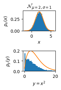
3. Delta Function

Consider a random variable with a probability density function (PDF) \(p_x(x)\). Let \(y = x^2\). The PDF \(p_y(y)\) is given by

\[\begin{gather*} p_y(y) = \int\delta(y - x^2)p_x(x)\d{x}. \end{gather*}\]

Compute this integral and determine \(p_y(y)\) in terms of the function \(p_x\).

4. Matrices

For each of the following types of matrices,

• Hermitian, Anti-hermitian, Unitary, Diagonal

state what this implies about:

1. The trace \(\Tr \mat{A}\).

2. The determinant \(\det \mat{A}\).

3. The adjoint \(\mat{A}^\dagger\)

4. The inverse \(\mat{A}^{-1}\).

5. A product of two such matrices \(\mat{A}\mat{B}\).

6. The eigenvalues and eigenvectors.

Example: Upper Triangular Matrix

For an upper triangular matrix:

1. Nothing is special about the trace.

2. The determinant is the product of the diagonals.

3. The adjoint is lower triangular.

4. The inverse is upper triangular.

5. The product is upper triangular.

6. The eigenvalues are the diagonal entries, and the eigenvectors can be organized into an upper triangular matrix.

Numerical example (not needed for your assignment):

\[\begin{gather*} \mat{A} = \begin{pmatrix} 1 & 2 & 3\\ 0 & 4 & 5\\ 0 & 0 & 6 \end{pmatrix}, \qquad \mat{A}^\dagger = \begin{pmatrix} 1 & 0 & 0\\ 2 & 4 & 0\\ 3 & 5 & 6 \end{pmatrix}, \qquad \det \mat{A} = 1\cdot 4\cdot 6 = 24,\\ \mat{A}^{-1} = \begin{pmatrix} 1 & -\frac{1}{2} & -\frac{1}{12}\\ 0 & \frac{1}{4} & -\frac{5}{24}\\ 0 & 0 & \frac{1}{6} \end{pmatrix},\qquad \mat{A}^2 = \begin{pmatrix} 1 & 10 & 31\\ 0 & 16 & 50\\ 0 & 0 & 36 \end{pmatrix},\\ \mat{A}\mat{V} = \mat{V}\mat{D}, \qquad \mat{D} = \begin{pmatrix} 1 & 0 & 0\\ 0 & 4 & 0\\ 0 & 0 & 6 \end{pmatrix},\qquad \mat{V} = \begin{pmatrix} 1 & 2 & 16\\ 0 & 3 & 25\\ 0 & 0 & 10 \end{pmatrix} \end{gather*}\]

5. Rotation Matrices

Hints: Consider the Pauli matrices. Also, note that rotation matrices can be expressed as \(\mat{R}_{\vect{\theta}} = e^{\mat{\vect{\theta}\times}}\).

Here \([\mat{A}, \mat{B}] = \mat{A}\mat{B} - \mat{B}\mat{A}\) is the commutator.

The effect of rotations on physical systems can be expressed in terms of Lie algebras and groups as we will discuss later in the course. For now, find examples of three 2D and 3D matrices \(\mat{T}_{x,y,z}\) that satisfy the following commutation relationships:

\[\begin{gather*} [\mat{T}_x, \mat{T}_y] = -\mat{T}_{z} \quad \text{and cyclic permutations:} \quad [\mat{T}_y, \mat{T}_z] = -\mat{T}_{x}, \quad [\mat{T}_z, \mat{T}_x] = -\mat{T}_{y}. \end{gather*}\]

Prove that the trace of any such matrices must be zero: \(\Tr\mat{T}_{i} = 0\). Show that if the matrices \(\mat{T}_{i}^\dagger = \pm\mat{T}_{i}\) are either hermitian or anti-hermitian, then they must be anti-hermitian: \(\mat{T}_{i}^\dagger = -\mat{T}_{i}\).

Can the matrices \(\mat{T}_{i}\) be real in 3D? What about 2D? Justify your answer.

Physicists typically include a factor of \(\I = \sqrt{-1}\) in the definition of the commutation relations, so you will often see

\[\begin{gather*} [\mat{M}_{i}, \mat{M}_{j}] = \I \epsilon_{ijk}\mat{M}_k,\qquad \mat{R}_{\theta} = e^{\I \vect{\theta}\cdot\vect{\mat{M}}}. \end{gather*}\]

Show how \(\mat{M}_{i}\) can be obtained from \(\mat{T}_{i}\).

Note

Armed with such matrices, one can form matrices that effect rotations on on spinors (2D) and vectors (3D) by exponentiating:

\[\begin{gather*} \mat{R}_{\vect{\theta}} = \exp\left(\sum_{i\in\{x,y,z\}} \theta_i \mat{T}_{i}\right) \equiv e^{\vect{\theta}\cdot\vect{\mat{T}}}. \end{gather*}\]

The linear combinations of \(\mat{T}_{i}\) form a representation of the Lie algebra \(\mathfrak{so}(3)\) and exponentiating these gives the rotation matrices, which form a representation of the corresponding Lie group \(SO(3)\). In the case of the 2D representation, this is related to the Lie group \(SU(2)\) (but the topology of these two groups differ as we will discuss later).