7. Ordinary Differential Equations (ODEs)

7. Ordinary Differential Equations (ODEs)#

There are a few special cases that are exactly solvable. Most tricks attempt to bring an equation into one of these forms. Note that there are many tricks, and so often it is easiest to try to use a table of exact results like [Polyanin and Zaitsev, 2018] if you need an exact solution. These notes are intended as a summary of Chapter 7 of [Arfken et al., 2013].

Separable#

\[\begin{gather*} P(x)\d{x} + Q(y)\d{y} = 0, \qquad \int_{x_0}^{x}P(x)\d{x} = \int_{y_0}^{y}Q(y)\d{y}. \end{gather*}\]

For most physics problems, I highly recommend including the endpoints of integration – this makes determining the constants of integration much more natural.

Exact#

\[\begin{gather*} \overbrace{ \underbrace{P(x,y)}_{\partial_x f}\d{x} + \underbrace{Q(x,y)}_{\partial_y f}\d{y} }^{\d{f}(x,y)=\partial_x f\d{x} + \partial_y f\d{y}} = 0,\qquad \overbrace{\partial_{y}\underbrace{P(x,y)}_{\partial_{x}f}}^{\partial_{yx}f} = \overbrace{\partial_{x}\underbrace{Q(x,y)}_{\partial_{y}f}}^{\partial_{xy}f},\\ f(x,y) = C. \end{gather*}\]

The idea here is to express the ODE as a total derivative of some function \(f(x, y)\) which will then be constant. A quick check is to look at the mixed partials to see if they are equal \(f_{,xy} = f_{,yx}\).

Integrating Factor#

Related is trying to find an integrating factor \(\lambda(x)\) such that multiplying the equation by it makes it exact:

\[\begin{gather*} \lambda(x)(P(x, y)\d{x} + Q(x, y)\d{y}) = \d{f} = 0, \qquad f(x, y)= C. \end{gather*}\]

Integrating factors always exist, but there is no general algorithm for finding them.

Example: General first-order linear equation.

Linear first-order equations always have a solution

\[\begin{gather*} y' + p(x)y = q(x). \end{gather*}\]

As [Arfken et al., 2013] shows, one can try to find an integrating factor that makes it exact.

Solution: Finding an Integrating Factor

To solve this by finding an integrating factor, note that we seek a function \(\lambda(x)\) such that

\[\begin{gather*} \lambda(x)(\d{y} + p(x) y\d{x}) = \d{f} \end{gather*}\]

is exact. If we can find such a function, then our ODE will be

\[\begin{gather*} \d{f} = \lambda(x)q(x)\d{x} \end{gather*}\]

which can be solved (expressed in terms of definite integrals):

\[\begin{gather*} f(x,y) = \int \lambda(x)q(x)\d{x}. \end{gather*}\]

Equating mixed partials gives the condition

\[\begin{gather*} \partial_{x}(\lambda) = \partial_y(\lambda p y)\\ \lambda' = \lambda p\\ \frac{1}{\lambda}\d{\lambda} = p(x) \d{x}\\ \lambda(x) = e^{\int^{x} p(x)\d{x}}. \end{gather*}\]

To find \(f(x, y)\), we can integrate the two terms

\[\begin{gather*} \lambda(x) = \partial_{y}f(x, y), \qquad \lambda(x)p(x) y = \partial_{x}f(x, y). \end{gather*}\]

The first implies

\[\begin{gather*} f(x, y) = y \lambda(x) + g(x). \end{gather*}\]

The second implies

\[\begin{gather*} \lambda(x)p(x) y = \partial_{x}f(x, y) = y\underbrace{\lambda'(x)}_{\lambda(x)p(x)} + g'(x). \end{gather*}\]

This leaves \(g(x) = C\) as an integration constant.

Thus, we have the general solution

\[\begin{gather*} \lambda(x) = e^{\int^{x}p(x)\d{x}},\\ f(x, y) = y \lambda(x) = \int^{x} \lambda(x) q(x)\d{x}\\ y(x) = \frac{\int^{x} \lambda(x) q(x)\d{x}}{\lambda(x)}. \end{gather*}\]

For example, consider

\[\begin{gather*} y' + 2xy = e^{-x^2}. \end{gather*}\]

The solution is

\[\begin{gather*} \lambda(x) = e^{\int^{x} 2x\d{x}} = e^{x^2}\\ y(x) = \frac{\int^{x} e^{x^2}e^{-x^2}\d{x}}{e^{x^2}} = (x+C)e^{-x^2}. \end{gather*}\]

As a check:

\[\begin{gather*} y(x) = (x+C)e^{-x^2}, \qquad y'(x) = \bigl(1 - 2x(x + C)\bigr)e^{-x^2},\\ y' + 2xy = \bigl(1 - 2x(x + C)\bigr)e^{-x^2} + 2x(x+C)e^{-x^2},\\ = e^{-x^2}. \end{gather*}\]

Isobaric/Homogeneous#

These are equations of the form

\[\begin{gather*} \diff{x}{y} = f(x,y), \qquad f(sx, s^{m}y) = s^{m-1}f(x, y). \end{gather*}\]

Basically, this means that the equation makes sense dimensionally, and that one can introduce a dimensionless variable \(v = y/x^{m}\) so \(y = vx^{m}\) to separate the equations:

\[\begin{gather*} y' = v'x^{m} + mv x^{m-1} = f(x, vx^m) = x^{m-1}f(1, v)\\ \frac{\d{v}}{mv - f(1, v)} + \frac{\d{x}}{x} = 0. \end{gather*}\]

The basic idea is that \(x\) and \(y\) have the “same” dimensions (up to a power \(m\)), and this just defines the units for the problem. Once these units are scaled out, we obtain a separable equation for the non-trivial dimensionless combination \(v\).

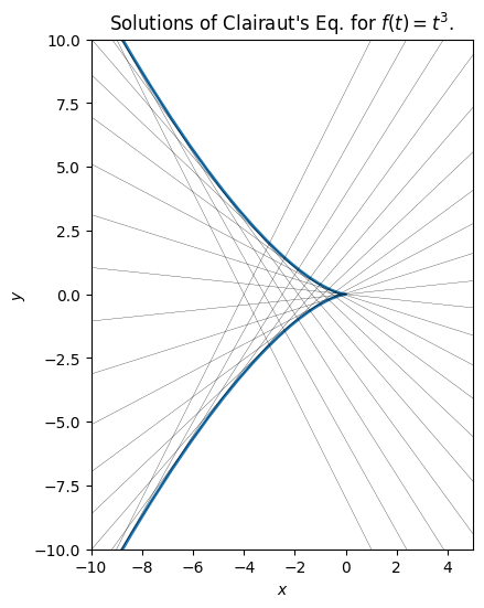
_images/04c5c81cacffee87dcdf2d5cbd6c9609c12ff911481d78a7fd1b216fee1e2813.png

Clairaut’s Equation: Envelopes#

A fun example worth being aware of is Clairaut’s Equation:

\[\begin{gather*} y - xy' = f(y'). \end{gather*}\]

Notice that this is solved by a general set of lines whose slopes and intercepts are related by \(b = f(m)\):

\[\begin{gather*} y(x) = mx + b, \qquad y - xy' = b = f(y') = f(m). \end{gather*}\]

The interesting property is that the envelope of these lines is also a singular solution of the equation. This can be found by differentiating the equation again:

\[\begin{gather*} y' - y' - xy'' = - xy'' = f'(y')y'', \qquad \Bigl(x + f'(y')\Bigr)y'' = 0. \end{gather*}\]

Thus, either \(y''=0\) – the lines we have already described – or \(x + f'(y') = 0\) – which describes the singular solution through the parametric relationship

\[\begin{gather*} x(m) = -f'(m), \qquad y(m) = f(m) - tf'(m) \end{gather*}\]

where \(m\) is the slope (which changes monotonically as we traverse the envelope).

Do It! Find the singular solution.

The equation \(x = -f'(y')\) suggests using \(t=y'(x)\) as a parameter so that \(x(t) = -f'(t)\). Differentiating \(y(t)\), we have

\[\begin{gather*} x(t) = -f'(t), \qquad \dot{x} = -f''(t), \qquad \dot{y}(t) = y'\dot{x} = -t f''(t), \\ y(t) = - \int^{t} tf''(t)\d{t} = -tf'(t) + \int^{t} f'(t)\d{t} = -tf'(t) + f(t) + C. \end{gather*}\]

It looks like we have an integration constant here, but remember that we are solving the derivative of the original equation. Returning to Clairaut’s Equation, we have

\[\begin{gather*} y' = \frac{\dot{y}}{\dot{x}} = \frac{-t f''(t)}{-f''(t)} = t\\ y - xy' - f(y') = -tf'(t) + f(t) + C + tf'(t) - f(t) = C = 0. \end{gather*}\]

Hence, the integration constant was spuriously introduced by our procedure and the solution is in fact singular.

Variation of Parameters#

Related to the method of undetermined coefficients used to solve \(y' + p(x)y = q(x)\) is Lagrange’s method of variation of parameters, which is useful for finding particular solutions of the inhomogeneous equation

\[\begin{gather*} y'' + p(x)y' + q(x)y = f(x) \end{gather*}\]

if you know the homogeneous solutions. I.e., let \(y_n(x)\) satisfy the homogeneous equation

\[\begin{gather*} y'' + p(x)y' + q(x)y = 0, \end{gather*}\]

then look for solutions that are linear combinations of the form

\[\begin{gather*} y(x) = u_1(x)y_1(x) + u_2(x)y_2(x). \end{gather*}\]

Dropping the explicit \(x\) dependence in further expressions, the trick is to impose the condition \(u_1'y_1 + u_2'y_2 = 0\) so that we have the following:

\[\begin{align*} y &= u_1y_1 + u_2y_2,\\ y' &= u_1y'_1 + u_2y'_2 + \smash{\overbrace{u'_1y_1 + u'_2 y_2}^{0}},\\ y'' &= \underbrace{u_1y''_1 + u_2y''_2}_{\text{will cancel}} + \underbrace{u_1'y'_1 + u_2'y'_2}_{\text{will remain}}. \end{align*}\]

Substituting these back into the original equation, the left set of terms cancel, and what remains, including the trick, is a solvable linear set of equations for \(u'_n(x)\):

\[\begin{align*} u_1'y_1 + u_2'y_2 &= 0,\\ u_1'y'_1 + u_2'y'_2 &= \frac{f(x)}{p(x)}, \\ \begin{pmatrix} y_1 & y_2\\ y'_1 & y'_2 \end{pmatrix} \begin{pmatrix} u_1' \\ u_2' \end{pmatrix} &= \begin{pmatrix} 0\\ f(x)/p(x) \end{pmatrix}, \\ \begin{pmatrix} u_1' \\ u_2' \end{pmatrix} &= \frac{1}{W} \begin{pmatrix} y'_2 & -y_2\\ -y'_1 & y_1 \end{pmatrix} \begin{pmatrix} 0\\ f(x)/p(x) \end{pmatrix}, \\ W &= \begin{vmatrix} y_1 & y_2\\ y_1' & y_2' \end{vmatrix} =y_1y_2' - y_2y_1'. \end{align*}\]

Note that this works for higher order equations: see [Polyanin and Zaitsev, 2018] for details.

Series and Frobenius’s Method#

The goal is to look for series solutions for ODEs. The general strategy is:

Look for singularities and asymptotic behaviour.
Express the solution as an appropriate series.
Find recurrence relations for the coefficients.
Check the solution for convergence, issues, and against the original equation.

To simplify matters, we will always expand about \(x=0\), but for a given differential equation it might make sense to expand about another point \(x_0\). If so, just change variables. Here are some notes:

1. Singularities and Asymptotics

[Arfken et al., 2013] describes the general approach for identifying singularities based on Fuch’s theorem. E.g., if we write the equation as

\[\begin{gather*} x^2 y'' + p(x) x y' + q(x) y = g(x), \end{gather*}\]

then there are no singularities where \(p(x)\), \(q(x)\), and \(g(x)\) are analytic.

Note

In [Arfken et al., 2013] and [Hassani, 2013], they consider

\[\begin{gather*} y'' + P(x) y' + Q(x) y = 0, \end{gather*}\]

and couch this in terms of \(P(x) = p(x)/x\) having at worst a simple pole, and \(Q(x) = q(x)/x^2\) having at worst a double pole.

One should also consider \(x \rightarrow 1/w\) to see if there are singularities at \(x\infty\).

Looking for the asymptotic behaviour is not generally considered a part of the Frobenius method, but can be very helpful for physical applications and is used extensively in quantum mechanics. For example, if we consider the following differential equation

\[\begin{gather*} -y'' + (x^2 - a) y = 0 \end{gather*}\]

which arises from the Schrödinger equation for a quantum harmonic oscillator, then we find that the solutions have the form

\[\begin{gather*} y(x) = e^{-x^2/2}H(x) \end{gather*}\]

where \(H(x)\) is a polynomial. I.e., factoring out the correct asymptotic behaviour renders the solution exact. Of course, there is no problem

Details

For large \(x\), we can neglect \(a\) to obtain

\[\begin{gather*} y'' \approx x^2 y. \end{gather*}\]

Looking for solutions that vanish for large \(x\), we see that \(y \approx e^{-x^2/2}\) is appropriate:

\[\begin{gather*} y' = -xy, \qquad y'' = -y-xy' = (x^2-1)y \approx x^2 y. \end{gather*}\]

Thus, we might consider series solutions of the form

\[\begin{gather*} y(x) = H(x)e^{-x^2/2}, \qquad H(x) = \sum_{n=0}^{\infty} a_{n}x^n. \end{gather*}\]

We will find that, for appropriate values of \(a\) (associated with the quantized energy eigenstates), the series terminates yielding the Hermite polynomials \(H(x)\).

Of course, there is nothing wrong with simply looking for a series solution for \(y(x)\) directly – it will be related to this by expanding the gaussian, but will have infinitely many terms.

2. Form of the Series

The standard approach is to write the solution as

\[\begin{gather*} y(x) = x^{s}\sum_{n=0}^{\infty} a_n x^n. \end{gather*}\]

The factor \(x^{s}\) has a similar flavour describing “asymptotic” behaviour that might not be of a pure power-law form. Additional factors deduced above might be included here.

In any case, the first task is to solve the indicial equation for \(s\) (called \(\nu\) in [Hassani, 2013]) by requiring that the first non-zero term is \(a_0\). If \(x=0\) is not singular as described above, then Fuch’s theorem ensures that there will be a solution of this form. In general, we expect a second order ODE to generate a quadratic indicial equation, and the two values of \(s \in \{s_1, s_2\}\) will generate the two independent solutions.

This can fail if the two solutions differ by an integer \(s_1 - s_2 \in \mathbb{Z}\) including zero (\(s_1 = s_2\)). In this case, the recurrence might fail to give an independent solution, but one can then look for a second solution \(y_2(x)\) of the form

\[\begin{gather*} y_1(x) = x^{s_1}\sum_{n=0}^{\infty} a_n x^n, \qquad y_2(x) = x^{s_2}\sum_{n=0}^{\infty} b_n x^n + C y_1(z) \ln z. \end{gather*}\]

Theorem 15.2.6 of [Hassani, 2013] states the precise conditions for this solution, which can also be found using the method of variation of parameters discussed above.