Monte Carlo

Hide code cell content

import mmf_setup;mmf_setup.nbinit()
import logging;logging.getLogger('matplotlib').setLevel(logging.CRITICAL)
%matplotlib inline
import numpy as np, matplotlib.pyplot as plt

This cell adds /home/docs/checkouts/readthedocs.org/user_builds/physics-571-math-methods/checkouts/latest/src to your path, and contains some definitions for equations and some CSS for styling the notebook. If things look a bit strange, please try the following:

  • Choose "Trust Notebook" from the "File" menu.
  • Re-execute this cell.
  • Reload the notebook.

Monte Carlo#

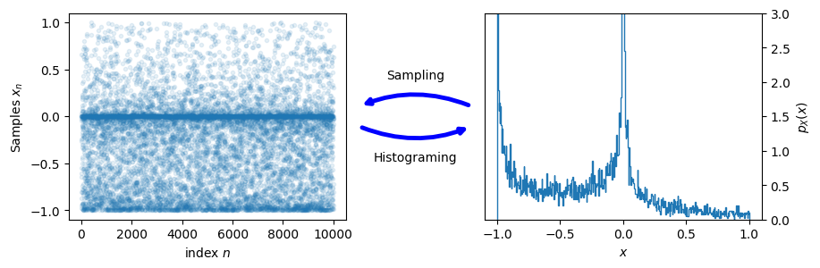
Here we describe how to represent probability distributions numerically with samples. For example, consider a single random variable \(X\) with PDF \(p_X(x)\). We can of course represent this by the function \(p_X(x)\), but this can be tricky, especially in higher dimensions.

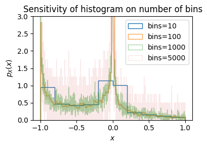
An alternative is to use a large set of samples \(\vect{x} = \{x_0, x_1, \dots, x_{N-1}\}\). To get back to the PDF we use a histogram.

Hide code cell source

# Random number generator
rng = np.random.default_rng(seed=2)

Ns = 10000   # Number of samples
u = rng.random(size=(Ns))  # Uniform distribution - boring
x = (2*u**2-1)**3          # Something more interesting

fig, ax = plt.subplots(figsize=(4,3))
for n, bins in enumerate([10, 100, 1000, 5000]):
    ax.hist(x, bins=bins, density=True, 
            histtype='step', label=f"{bins=}", 
            alpha=1-0.9*n/3)
ax.legend()
ax.set(xlabel="$x$", ylabel="$p_X(x)$", ylim=(0, 3),
       title="Sensitivity of histogram on number of bins")
plt.tight_layout()
../_images/fa25e1004fda50b9f75a00bfa1ebd71459409aa4fa74d8ec77006768496f5615.png

Hide code cell source

fig, axs = plt.subplots(1, 2, figsize=(10, 3), gridspec_kw=dict(wspace=0.5))
ax = axs[0]
n = np.arange(len(x))
ax.plot(n, x, '.', alpha=0.1)
ax.set(xlabel="index $n$", ylabel="Samples $x_n$")

ax = axs[1]
ax.hist(
    x, 
    bins=500,        # How many bins -- choose carefully.
    density=True,    # Normalize the PDF
    histtype='step') # Looks better to me.

ax.set(xlabel="$x$", ylabel="$p_X(x)$", ylim=(0, 3))
ax.yaxis.set_label_position("right")
ax.yaxis.tick_right()

for xy, xytext, text in [((1.05, 0.55), (1.45, 0.55), "Histograming"),
                         ((1.45, 0.45), (1.05, 0.45), "Sampling")]:
    axs[0].annotate(xy=xy, xytext=xytext, text="", xycoords='axes fraction',
                    arrowprops=dict(arrowstyle='->',
                                    connectionstyle='arc3,rad=0.2',
                                    color='blue',
                                    lw=3.5,
                                    ls='-'));
    x = (xy[0] + xytext[0])/2
    y = xy[1] + 5*(0.5 - xy[1])
    axs[0].text(x, y, text, transform=axs[0].transAxes, ha='center', va='center')
../_images/d1ea6aaf98aae0019ebdd0f3b9e202634ea8ee29577574aba11d38502ea82de6.png

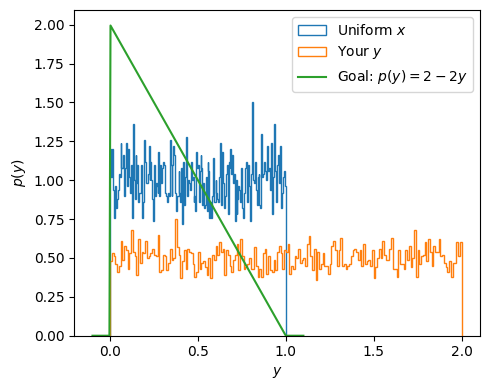
Do It! How do you sample a given PDF \(p(y)\) from a uniform sample?

Given a set \(\vect{x}\) uniformly sampled from the interval \(x\in [0, 1]\), how can you transform them \(y=f(x)\) to sample a desired PDF \(p(y)\)? Test your answer with the code below. Try to get samples with the following PDF:

\[\begin{gather*} p(y) = \begin{cases} 2(1-y) & y \in [0, 1]\\ 0 & \text{otherwise} \end{cases} \end{gather*}\]
# Random number generator - seed for reproducibility
rng = np.random.default_rng(seed=2)

Ns = 10000   # Number of samples
x = rng.random(size=(Ns))  # Uniform distribution

# Your answer goes here ####
y = 2*(1-x)

@np.vectorize
def p(y):
    if y < 0 or y > 1:
        return 0.0
    return 2*(1-y)

fig, ax = plt.subplots(figsize=(5,4))
ax.hist(x, bins=200, density=True, histtype='step', label="Uniform $x$")
ax.hist(y, bins=200, density=True, histtype='step', label="Your $y$")
y_ = np.linspace(-0.1, 1.1, 200)
ax.plot(y_, p(y_), label="Goal: $p(y) = 2-2y$")
ax.legend()
ax.set(xlabel="$y$", ylabel="$p(y)$")
plt.tight_layout();
../_images/47cdbd3e68edd482159f7a9d464465cb11e796d7abae4b6324cf16073a756ba3.png