23. Probability#
Motivating Problems#
Consider a room with \(N\) people. Whbat is the probability \(P\) that two of them share the same birthday?
How many different rooms of \(N\) people would you need to sample in order to get a good empirical estimate of \(P\)?
Suppose you have a coin that gives heads with probability \(p\) and tails with probability \(1-p\). How many flips \(N\) would you need to establish \(p\) to within \(\pm 0.1\) with 95% confidence?
Questions and Misconceptions#
Consider a biased coin that lands heads twice as often as tails. Is this coin random?
Solve the standard Monty Hall problem. (Some people – apparently including Paul Erdős – find this confusing, but I don’t really understand why.)
Suppose that you see photons from a star that explodes at time \(t_0\) and that the probability of measuring these photons has a known probability density (PDF)
\[\begin{gather*} p(t) = \alpha \Theta(t-t_0)e^{-t/\tau} = \begin{cases} \alpha e^{-t/\tau} & t > t_0,\\ 0 & t < t_0, \end{cases} \end{gather*}\]where \(\alpha\) is chosen to normalize the distribution and \(\tau\) is known (we will take \(\tau = 1\) as defining our units for time). What can you say about the time \(t_0\) if three photons are observed at times \(t/\tau \in \{12, 14, 16\}\)? Formally, determine a 90% CI for \(t_0\). (See Warmup 2: Recognizable Subclasses for details.)
Background#
Dirac Delta Function#
Evaluate the following with a change of variables:
where the sum runs over all points \(x_i\) that satisfy the condition.
Probabilities and PDFs#
A key idea is that if \(n\) of \(N\) equally likely cases satisfy some condition, then the probability associated with that condition is \(p = n/N\), so, in principle, once can just count. (But counting is often hard!)
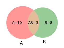
To get things straight, consider a bag containing \(N=15\) balls with the following properties:
\(N_A = 10\) have the letter “A” written on them.
\(N_B = 8\) have the letter “B” written on them.
\(N_{AB} = 3\) have both the letters “A” and “B” written on them.
Now we can consider the following probabilities for drawing balls randomly:
\(P(A \cap B) = N_{AB}/N = 3/15\): The probability of drawing a ball with letters “A” and “B”.
\(P(A \cup B) = N/N = 1\): The probability of drawing a ball with letters “A” or “B”.
\(P(A) = N_A/N = 10/15\): The probability of drawing a ball with the letter “A”.
\(P(B) = N_B/N = 8/15\): The probability of drawing a ball with the letter “B”.
Now for the conditional probability:
\[\begin{gather*} P(A | B) = \frac{P(A \cap B)}{P(B)} = \frac{3}{8}, \qquad P(B | A) = \frac{P(A \cap B)}{P(A)} = \frac{3}{10}. \end{gather*}\]You should think of \(P(A|B)\), read as “the conditional probability of A given B”, or “the probability of A under the condition B” as: What fraction of all the balls that have a “B” on also have an “A” on them?
From this, we can solve for \(P(A \cap B)\) in both cases:
\[\begin{gather*} P(A | B)P(B) = P(B|A)P(A) = P(A \cap B). \end{gather*}\]This gives Bayes’ Theorem:
\[\begin{gather*} P(A | B) = \frac{P(B|A)P(A)}{P(B)}. \end{gather*}\]The useful interpretation of this for physics is as follows:
Often one can get quite far by describing the problem. If events \(A\) and \(B\) are disjoint and have probabilities \(P_A\) and \(P_B\) respectively, then, the probability of:
\(A\) and \(B\) occurring is \(p = P_AP_B\): i.e. since both \(A\) and \(B\) must occur, the outcome is less likely: \(p = P_AP_B \leq P_A, P_B\).
\(A\) or \(B\) occurring is \(p = P_A + P_B\): i.e. allowing for both outcomes makes the outcome more likely: \(p = P_A + P_B \geq P_{A}, P_{B}\).
These concepts carry over to continuous variables where the probabilities are replaced by a probability density function (PDF) \(p(x)\) and the probabilities follow by integrating over appropriate regions of space:
\[\begin{gather*} P_A = \int_{A}p(x)\d{x}, \qquad P_B = \int_{B}p(x)\d{x}, \end{gather*}\]etc. In this language, we can view \(A\) and \(B\) as subsets of our space. The notion of disjoint means that the intersection is empty: \(A \cup B = \emptyset\). (More technically, \(A \cup B\) has zero measure.)
Random Variables#
(See Random Variables for more details.)
A random variable is a quantity \(X\) that can randomly take different values \(x\) according to a PDF \(p_X(x)\).
Note
On our motivating problem, we have at least three random variables:
\(B \in \{1, 2, \dots 365\}\): The birthday of a random person in the room. We assume this has a fixed distribution.
\(S_2 \in \{0, 1\}\): the outcomes of the experiment. Either two people have the same birthday (\(S_2 = 1\)), or no one does \(S_2 = 0\).
\(P_{t} \in \{0, 1/t, 2/t, \cdots 1\}\): The mean after running \(t\) trials.
Parameter Fitting#
Here we try a simple problem of determining the drag coefficient for an object falling in a gravitational field. Here we will assume quadratic drag (see below for a more thorough example). We will start at height \(z=0\) with no velocity \(\dot{z}=0\) at time \(t=0\):
Do It! Derive \(z(t)\).
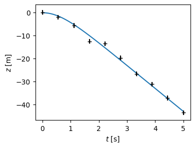
Now let’s simulate some measurements. Suppose we can measure the position, but with an uncertainty \(\sigma = 2\)m. For now we shall assume that the error is a normally distributed random variable:
m = s = 1.0       # SI Units

# Parameter values: these are the "truths" in our simulations
v_t = 10.0*m/s    # Terminal velocity
g = 9.8*m/s**2    # Acceleration due to gravity

# Here is the function we are fitting.  We use the true values as the defaults
def f(t, v_t=v_t, g=g):
    """Return the height of a falling particle at time t."""
    return -v_t**2/g * np.log(np.cosh(g*t/v_t))

T = 5.0*s
Nt = 10  # Number of data points.

ts = np.linspace(0, T, Nt)
sigma = 1.0 * np.ones(len(ts))       # Constant errors +-1.0m
rng = np.random.default_rng(seed=2)  # Always seed so you can reproduce results

# Simulate some gaussian measurement errors
eps = rng.normal(scale=sigma, size=Nt)
xdata = ts
ydata = f(ts) + eps
yerrs = np.ones(len(ts)) * sigma

fig, ax = plt.subplots(figsize=(4, 3))
t = np.linspace(0, T)
ax.plot(t, f(t))
ax.set(xlabel="$t$ [s]", ylabel="$z$ [m]");
ax.errorbar(xdata, ydata, yerr=yerrs, fmt='+k');
Curve Fit#
We start by doing a normal least-squares fit using scipy.optimize.curve_fit():
from scipy.optimize import curve_fit
params, pcov = curve_fit(f, xdata, ydata, p0=(v_t, g), sigma=yerrs, absolute_sigma=True)
chi2 = float(sum(((f(xdata, *params) - ydata)/yerrs)**2)/2)
chi2r = chi2/(len(ydata) - len(params) - 1)
print(f"{params=}")
print(f"{pcov=}")
print(f"{chi2r=}")
params=array([ 9.88257299, 10.00280964])
pcov=array([[ 0.13532362, -0.41423092],
       [-0.41423092,  1.59471427]])
chi2r=0.8513317044888767
These are the parameter estimates \(\vect{\theta}_0 \) where \(\vect{\theta}^T = (v_t, g)\), the corresponding covariance matrix \(\mat{C}\), and the reduced \(\chi^2\) of the fit. The interpretation is that the errors \(\vect{\epsilon} = \vect{\theta} - \vect{\theta}_0\) parameters are described by the following multi-normal PDF:
Interpreting \(\mat{C}\).
We can interpret the diagonals of \(\mat{C}^{-1}\) and \(\mat{C}\) as the squares of the errors in the parameters. Consider a single parameter. From the property above we see that the corresponding \(1/\diag{\mat{C}^{-1}}\) gives the variance in that parameter holding all the other parameters fixed.
A little less obvious is the meaning of \(\diag{\mat{C}}\) as the variance of the parameter while marginalizing over the other parameters – i.e., imaging adjusting the parameter you are studying, but then re-fitting the other parameters. As a quick check, the latter should be larger than the former.
print(1/np.sqrt(np.diag(np.linalg.inv(pcov))))
print(np.sqrt(np.diag(pcov)))
[0.16651165 0.57160927]
[0.36786359 1.26281997]
For simplified analyses at the level of assuming errors are gaussian and small enough that the functions can be treated as linear, there is a nice package uncertainties that does forward error propagation with correlated errors using automatic differentiation.
import uncertainties
v_t_, g_ = uncertainties.correlated_values(params, pcov)
print(f"{v_t_ = :S}, {g_ = :S}")
v_t_ = 9.9(4), g_ = 10.0(1.3)
We see that these errors correspond to the marginalized uncertainties \(\sqrt{\diag{\mat{C}}}\).
If your errors are small enough that the model is effectively linear over the region of interest and your errors are gaussian, then you can stop here and use these results (but be careful about reporting the confidence region - see [Press et al., 2007]). Otherwise, you should check this with MCMC.
Bayesian Fitting with MCMC#
The key challenge of Bayesian analysis is to express the likelihood: the probability \(p(x|\theta)\) of getting the data \(x\) given fixed values of the parameters \(\theta\). To do this, ask yourself – what is the source of the uncertainty?
Here it is the random variable \(\epsilon_i\) characterizing the errors, so
Uncertainties in the Abscissa \(t_i\).
The formulation here codifies uncertainties in the measured heights \(z_i\) – the dependent variable or ordinate. What if we have uncertainties in the independent variable or abscissa \(t_i\)? Following the same logic, we should now write
We can interpret this in several ways:
We can think of \(t_i\) as parameters that we include in \(\theta\): these are the chosen values at which we try to run our experiment, but the actual measurements are effected randomly according to \(p_t(t_i)\).
Similarly, but you can think of \(p_t(t_i)\) as priors on the chosen time.
We can continue with our analysis as if the \(t_i\) are fixed, but then marginalize over the uncertainties by integrating over \(t_i\):
\[\begin{gather*} \int p(x|\theta)p_t(t_i)\d t_i. \end{gather*}\]Note: we recover our fixed abscissa results if we take \(p_t(t_i) = \delta(t_i - \tilde{t}_i)\).
We proceed by including priors \(p(\theta)\), then using MCMC to sample the posterior
distribution. The usual least-squares approach is recovered if
\(p_{\epsilon}(\epsilon_i)\) is gaussian, and if we choose flat priors \(p(\theta)\propto
1\). Matching our choice of bounds above, we might choose flat priors within a given
range. Numerically, the MCMC code in emcee package requires a function that
computes the logarithm of the posterior:
import emcee

def log_probability(q, x, y, dy, g=g):
    """Return the log of the posterior probability.

    Arguments
    ---------
    q : (alpha, v_t)
        Array of parameters to be sampled.
    x, y, dy : array-like
        Arrays of the data points `(x, y)` and the y-errors `dy`.

    This code assumes uninformed uniform priors on the parameters, and that the errors
    are normally distributed with standard deviation `dy`.
    """
    v_t, g = q

    # Here are the priors: they are flat (log=0) but negative infinite
    # outside the allowed range (-inf = log(0)).  If we are outside the
    # allowed range, we bail so we don't accidentally pass invalid parameters
    # to f when we compute the log_likelihood.
    #
    # Note: you can try omitting these, but if the problem is difficult,
    # you might not get good results (usually seen as poor autocorrelation times).

    if v_t <= 0 or v_t > 400*m/s:
        return -np.inf

    if g <= 5*m/s**2 or g >= 30*m/s**2:
        return -np.inf

    log_prior = 0

    y_model = f(x, v_t=v_t, g=g)
    y_err = y - y_model

    # This is simply the log of the gaussian
    log_likelihood = np.sum(-0.5 * (y_err / dy)**2)

    log_prob = log_prior + log_likelihood
    return log_prob

# Get our initial state.  We initialize 32 initial "walkers".
Nwalkers, Nparams = 32, len(params)

# Use our previous parameter estimates to seed the walkers.
q0 = np.array(params) + 0.1*rng.normal(size=(Nwalkers, Nparams))

# Make sure all of our initial data is feasible... if you tighten the
# priors, you must make sure all q0 lie in a feasible region.
for q in q0:
    assert log_probability(q, xdata, ydata, yerrs) > -100

# Now create the sampler and generate some samples
sampler = emcee.EnsembleSampler(nwalkers=Nwalkers, ndim=Nparams,
                                log_prob_fn=log_probability,
                                args=(xdata, ydata, yerrs))
res = sampler.run_mcmc(initial_state=q0, nsteps=5000)

# Check the autocorrelation times.  We should use this to discard the initial samples,
# and thin the remaning samples for analysys
tau = sampler.get_autocorr_time()
print(tau)
[35.68495952 37.6997059 ]
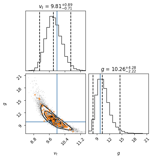
Now we inspect the results using a corner plot:
flat_samples = sampler.get_chain(discard=int(3*np.max(tau)), thin=int(np.mean(tau)/2), flat=True)

import corner
fig = corner.corner(flat_samples, labels=[r"$v_t$", r"$g$"],
                    truths=[v_t, g],
                    quantiles=[0.025, 0.5, 0.975],
                    #levels=[0.68, 0.95],   # You can adjust the contours here.
                    show_titles=True);


from IPython.display import display, Math

for ci in [68, 95]:
    res = [fr"{ci}\% \mathrm{{ CI}}:"]
    for n, name in enumerate(["v_t", "g"]):
        quantiles = [50 - ci/2, 50, 50 + ci/2]
        mcmc = np.percentile(flat_samples[:, n], quantiles)
        q = np.diff(mcmc)
        txt = r"\mathrm{{{3}}} = {0:.2f}_{{-{1:.2f}}}^{{{2:.2f}}}"
        res.append(txt.format(mcmc[1], q[0], q[1], name))
    display(Math(r" \qquad ".join(res)))
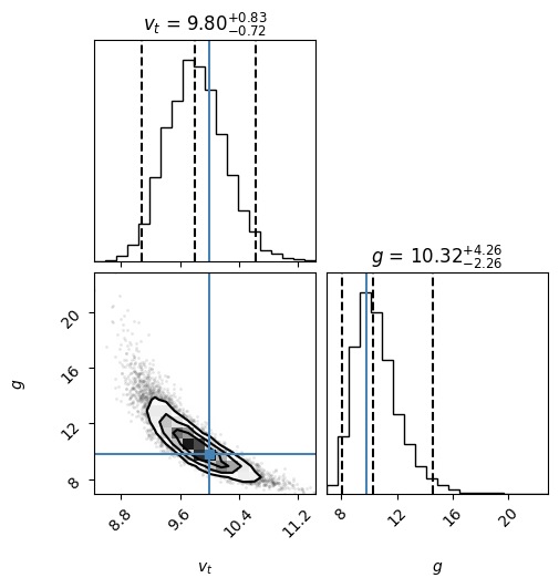
Notice that our estimates from scipy.optimize.curve_fit() \(v_t = 9.9(4)\)m/s and
\(g=10.0(1.3)\)m/s\(^2\) were pretty good in this case, corresponding to roughly a 1\(\sigma\) or
68% credible interval. Extending these to 95%, however, would significantly
underestimate the errors in \(g=10.0(2.6)\)m/s\(^2\) for example. This is partly because
the correlation between the parameters is not simple – it is somewhat banana-shaped.
These results could be carefully reported by:
Stating the marginalized values listed above and stating that the values quote are the median (50% quantile) with errors giving the 2.5% and 97.5% quantiles respectively.
Alternatively, you could compute symmetric confidence regions, or highest posterior density (HPD) credible intervals. The latter would mean the set \(A = \{θ \mid p(θ | x) \geq k\}\) where \(k\) is the largest real number such that \(P(A) \geq 0.95\). These are more difficult to compute in 1D, but natural in higher dimensions (see below).
Showing the corner plot, but being very careful about the meaning of the contours. Note that the contours here must be carefully interpreted. They are HPD credible sets, but the default levels in the 2D histogram contain 39.3% and 86.4% of the samples for \(1\sigma\) and \(2\sigma\) respectively. These tend to correspond well with the 1D CIs given above. If you want the true 68% or 95% regions, you can use the
levelsargument.
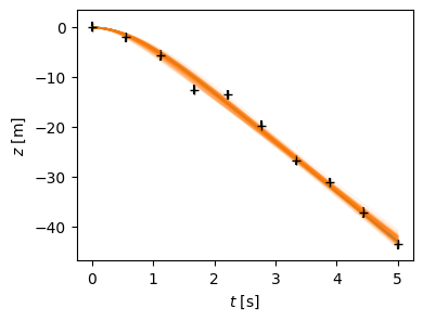
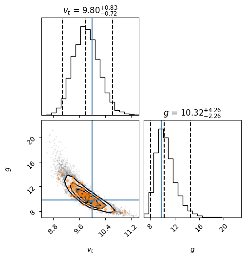
Finally, we can plot the data, and a bunch of the sampled trajectories. With a suitable choice of alpha-blending, this provides a nice way of visualizing the fit. We also plot these on the corner plot.
fig, ax = plt.subplots(figsize=(4, 3))
t = np.linspace(0, T)
ax.plot(t, f(t))
ax.set(xlabel="$t$ [s]", ylabel="$z$ [m]");
ax.errorbar(xdata, ydata, yerr=yerrs, fmt='+k');

# Now plot 100 random samples on top
inds = np.random.randint(len(flat_samples), size=100)
for ind in inds:
    sample = flat_samples[ind]
    ax.plot(t, f(t, *sample), "C1", lw=1, alpha=0.1)

fig = corner.corner(flat_samples, labels=[r"$v_t$", r"$g$"],
                    truths=[v_t, g],
                    quantiles=[0.025, 0.5, 0.975],
                    #levels=[0.68, 0.95],   # You can adjust the contours here.
                    show_titles=True);
ax = fig.get_axes()[2]  # This is a little tricky.  Must guess which is the main plot.
ax.plot(*(flat_samples[inds].T), '.C1', alpha=0.5);

Complete Code#
Here is the complete code for you to use as a starting point for another analysis: