Class Log - 2024#
These are notes about what we did in class in the Fall 2024 offering of the course.
Fri 11 Oct 2024#
Finite difference and drums.
Start complex analysis.
Wed 9 Oct 2024#
Review midterm exam.
Separation of variables in PDEs.
Explicit example of Drum.
Mon 7 Oct 2024#
Midterm I Exam
Fri 4 Oct 2024#
PDEs. Method of characteristics. Traffic flow.
Fri 4 Oct 2024#
Green’s functions: 1D Oscillator
\[\begin{gather*} \mathcal{L}u = \ddot{u} + 2\gamma \dot{u} + \omega_0^2 u = g(t). \end{gather*}\]Homogeneous solutions (assuming \(\gamma^2 < \omega_0^2\)):
\[\begin{gather*} u(t) = e^{-\gamma t} \Bigl(a_+ e^{\I\omega t} + a_-e^{-\I\omega t}\Bigr),\qquad \omega = \sqrt{\omega_0^2 - \gamma^2}. \end{gather*}\]Green’s function:
\[\begin{gather*} \mathcal{L}G(t) = \delta(t). \end{gather*}\]Construct from homogeneous solutions with appropriate discontinuity at \(t_0\). Many ways to do this, but the following is easy:
\[\begin{gather*} G(t) = \Theta(t)e^{-\gamma t}\frac{\sin(\omega t)}{\omega}. \end{gather*}\]
Mon 29 Sept 2024#
Variational Method
PDEs
Method of Characteristics.
Flow.
Separation of Variables.
Green’s functions.
Emphasize nature of solution. B/C.
Wave equation.
Fri 27 Sept 2024#
Sturm Liouville
Self-Adjoint
Hermite example.
Wed 25 Sept 2024#
Series Solutions:
Singularities.
Recurrence
Wronskian
Independence of solutions
Linear Equations
Reduction of order
Homogeneous
Inhomogeneous (Green’s functions)
Numerical tests
Mon 23 Sept 2024#
ODEs:
Separable
\[\begin{gather*} A(x)\d{x} = B(y)\d{y} \end{gather*}\]Exact
\[\begin{gather*} P(x, y)\d{x} + Q(x, y)\d{y} = 0, \qquad P = \varphi_{,x}, \qquad Q = \varphi_{,y}, \qquad P_{,y} = Q_{,x}, \qquad \varphi = \int_{x_0}^{x}P(x, y)\d{y} + \int_{y_0}^{y}Q(x_0, y)\d{y} = C. \end{gather*}\]First Order
Integrating Factors
Method of Variable coefficients
Series
Fri 20 Sept 2024#
Tensor summary. Note: I have made significant updates to 4. Tensors and Manifolds that I strongly encourage students read (especially the “Important” notes).
Wed 18 Sept 2024#
Tensors: Followed notes 4. Tensors and Manifolds up to the definition of the metric.
Discussed problem of computing \(\norm{\op{L}^2}^2\) and the role of Christoffle symbols (but briefly).
Students asked questions about matrices: especially the transpose, the difference between components and the actual “things” (I did not make this too explicit.)
Mentioned curves as vectors, and derivations as vectors but no details.
Mon 16 Sep 2024#
Tensors:
Vectors \(\ket{A} \equiv A_{\mu}\) and co-vectors \(\bra{A} \equiv A^{\mu}\).
Fields: \(A_{\mu}\).
Transformations: representations of rotations etc.
Inverse picture of transformations that leave the inner product invariant.
Lorentz.
Connection: Example from quantum mechanics.
\[\begin{gather*} \vect{\Psi}(\vect{x}) \rightarrow \mathcal{R}\vect{\Psi}(\vect{x}) = \mat{R}\vect{\Psi}(\mat{R}^{-1}\vect{x}),\\ \Psi^{a} \rightarrow [\mat{R}]^{a}{}_{b}\Psi^{b}. \end{gather*}\]\(\mat{1}\): \([\mat{1}]^{i}{}_{j} = \delta^{i}{}_{j} = \delta^{i}_{j}\) since \(\mat{1} = \mat{1}^T\).
Metric raises indices.
Fri 13 Sep 2024#
Finite differences and Hermitian vs. self-adjoint. (Working with functional operators.)
Vector Calculus:
Pictures. \begin{align*} \int_V \vect{\nabla}\cdot\vect{A}\d{\tau} & = \oint_{\partial V} \vect{A}\cdot\d{\vect{\sigma}},\ \int_S \vect{\nabla}\times\vect{B}\cdot\d{\vect{\sigma}} &= \oint_{\partial S} \vect{B}\cdot\d{\vect{r}},\ \oint_{C} \vect{\nabla} f \cdot \d{\vect{r}} &= \int_{\partial C} \d{f}. \end{align*}
Curvilinear coordinates (keep orthonormal frame)
Metric
Wed 11 Sep 2024#
Angular momentum: passive vs. active transformations. (Translation as an example.)
Eigenvalue problem. Diagonalization. Simultaneous Diagonalization.
Hermitian vs self-adjoint. Use finite difference operator as example.
\(L_2\) (see [Hassani, 2013] chapter 7, Thms. 7.2.1-7.2.3
Riesz-Fischer: \(\mathcal{L}^2_{w}(a,b)\) is complete.
All complete inner product spaces with countable bases are isomorphic to \(\mathcal{L}^2_{w}(a,b)\).
Stone-Weierstrass: \(\bigl\{x^n \mid n \in \{0, 1, 2, \dots\}\bigr\}\) forms a basis for \(\mathcal{L}^2_{w}(a,b)\).
Pauli matrices.
Mon 9 Sep 2024#
Completeness. Fourier space.
Angular momentum operators and function.
Fri 6 Sep 2024#
Direct sum and tensor product:
\(R_z = e^{\mat{\vect{\theta}\times}}\). Is this active or passive?
Groups: addition of angular momentum as an example.
Fourier transformation as change of basis.
Wed 4 Sep 2024#
Determinants and Matrices.
Vector spaces and Inner Product spaces.
Gram Schmidt
Vectors.
Orthogonal Polynomials
Completeness.
Projections.
Matrix factorization.
\(LU\): Gauss-Jordan Elimination (Solving systems)
\(LL^T\): Cholesky decomposition (stable version for symmetric matrices)
\(QR\): Gram-Schmidt Orthonomalization
\(SDS^{-1}\): Diagonalization, eigenvalues.
\(UDU^\dagger\): For Hermitian/Symmetric matrices
\(UDV^\dagger\): Singular Value Decomposition (SVD).
Example: Entanglement (Schmidt decomposition)
For details, see Linear Algebra.
Fri 30 Aug 2024#
Sequence acceleration.
Subtract a nearby sequence that you know the answer too (perhaps an integral)?
Partial fractions. (did not discuss)
Euler. (mentioned - see notes)
Weierstrauss and Abel test example.
E.g. Apply Abel test for \(e^{x}\) on \(x \in [0, 1]\). (did not do.)
Mathematical Induction.
Use induction to prove that $f(N) = \sum_{n=1}^{N} n = N(N+1)/2.
To get answer: Consider integral \(\int_{1}^{\infty}n\d{n} = (N^2-1)/2\).
Guess \(f(N) = a + bN + cN^2\).
Solve the following to get \(a=0\), \(b=c=1/2\):
\[\begin{gather*} f(1) = a + b + c = 1\\ f(2) = a + 2b + 4c = 3\\ f(3) = a + 3b + 9c = 6 \end{gather*}\]Prove by induction:
The formula works for a base case \(f(1) = 1\).
Note that \(f(N+1) = f(N) + N+1\).
If \(f(N) = N(N+1)/2\), then the latter implies
\[\begin{gather*} f(N+1) = \frac{N(N+1)}{2} + N+1 = \frac{N^2 + 3N + 2}{2} = = \frac{(N+2)(N+1)}{2}. \end{gather*}\]Hence our formula works for \(N+1\). Therefore it is correct for all integer \(N\geq 1\) by induction.
Derivatives
Extrema. (did not do)
Differentiate Parameters:
\[\begin{gather*} I_n = \int x^n e^{-x^2}. \end{gather*}\]
Delta function. (started)
Suppose two random variables \(X\) and \(Y\) have PDF \(p_X(x)\) and \(p_Y(y)\). What is the PDF for \(Z = X+Y\)?
Warmup: From intro physics lab, if \(x = \bar{x} \pm \sigma_x\) and \(y = \bar{y} \pm \sigma_y\) where \(\sigma_{x,y}\) are the standard deviations (“errors”), what is the standard deviation (“error”) \(\sigma_z\) in \(z = x+y\)?
Answer: \(\sigma_z = \sqrt{\sigma_x^2 + \sigma_y^2}\). Prove this. (Apparently this is no longer common knowledge.)
Wed 28 Aug 2024#
Power series.
Integration and differentiation.
\[\begin{gather*} f(x) = \frac{1}{2!} + \frac{2}{3!} + \frac{4}{5!} + \cdots. \end{gather*}\]\[\begin{gather*} f(x) = \frac{1}{1\cdot2} + \frac{x}{2\cdot 3} + \frac{x^2}{3\cdot 4} + \frac{x^3}{4\cdot 5} + \cdots. \end{gather*}\]
Binomial expansion. Example: \(E = \sqrt{m^2c^4 + p^2c^2} = mc^2 + \tfrac{1}{2}mv^2 + \cdots\).
Weierstrauss and Abel tests.
Mention \(\delta(x)\).
Mon 26 Aug 2024#
Review of better method of series convergence: integral test + generalized ratio test. See notes in 1. Mathematical Preliminaries.
Fri 23 Aug: Series#
Convergence: Metric spaces; Cauchy convergence; \(\mathbb{R} = \) Cauchy completion of \(\mathbb{Q}\); Absolute vs. Conditional.
Common Series:
Harmonic (divergent):
\[\begin{gather*} \sum_{n=1}^{\infty} \frac{1}{n} = \frac{1}{1} + \frac{1}{2} + \frac{1}{3} + \frac{1}{4} \dots. \end{gather*}\]Geometric (convergent for \(0 \leq \abs{r} < 1\)):
\[\begin{gather*} \sum_{n=1}^{\infty} \frac{1}{r^n} = 1 + r + r^2 + r^3 = \dots = \frac{1}{1-r}. \end{gather*}\]Riemann Zeta function shows up in various places, and has known values for even integers:
\[\begin{gather*} \zeta(s) = \sum_{n=1}^{\infty} \frac{1}{n^s}, \qquad \zeta(2) = \frac{\pi^2}{6}, \qquad \zeta(4) = \frac{\pi^4}{90}, \end{gather*}\]and some other particular values.
Series Convergence Tests:
Integral test; Comparisons; Kummer/Gauss’s tests are more sensitive.
Proof of Ratio and Kummer tests; Telescoping Series; Enhanced Gauss’s test.
Series of Functions:
Uniform (sketch example 1.2.1); Independent concept from absolute convergence.
Weierstrass \(M\) Test (only for absolutely convergent series).
Abel’ Test.
Taylor Series (Mclauren series are about \(x=0\)).
Power Series; \(e^x\);
Can be integrated or differentiated (unlike Fourier series)
Unique; Formal power series. \begin{gather*} e^{x} = 1 + \frac{x}{1!} + \frac{x^2}{2!} + \cdots\ e^{\I x} = \underbrace{\left(1 - \frac{x^2}{2!} + \frac{x^4}{4!} - \cdots\right)}{\cos x} + \I\underbrace{\left(x - \frac{x^3}{3!} + \frac{x^5}{5!} - \cdots\right)}{\sin x} \end{gather*}
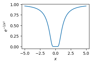
Consider \(f(x) = \exp(-1/x^2)\). All derivatives at \(x=0\) are zero: \(f^{(n)}(0) = 0\), but the function is \(C^{\infty}\) – infinitely smooth but very very flat!
Wed 21 Aug 2024#
Introductions.
Poll: who is interested in the mathematical theory (Hassani)? Roughly half the class.
Small problem:
\[\begin{gather*} a + b + c = 0\\ a^2 + b^2 + c^2 = \sqrt{74}\\ a^4 + b^4 + c^4 = ? \end{gather*}\]Discussed geometric picture a bit, connected (roughly) with \(L_p\) norm.
Discussed vector spaces: Most people know.
Inner product spaces: Some confusion. (E.g. Notion of angle in complex spaces?)
Gram-Schmidt: Not everyone knows.
Mentioned that functions are vectors.
\[\begin{gather*} \braket{f|g} = \int \d{x} f^*(x) g(x) \textcolor{green}{w(x)}. \end{gather*}\]Unifies fourier, orthogonal polynomials, many special functions, etc.
Discussed how to learn: how I learn.
Quick review of Syllabus, reading assignment.