Hide code cell content

import mmf_setup;mmf_setup.nbinit()
import logging;logging.getLogger('matplotlib').setLevel(logging.CRITICAL)
%matplotlib inline
import numpy as np, matplotlib.pyplot as plt

This cell adds /home/docs/checkouts/readthedocs.org/user_builds/physics-571-math-methods/checkouts/latest/src to your path, and contains some definitions for equations and some CSS for styling the notebook. If things look a bit strange, please try the following:

  • Choose "Trust Notebook" from the "File" menu.
  • Re-execute this cell.
  • Reload the notebook.

Assignment 5: ODEs#

Due Mon 29 Sept 2025 at the start of class

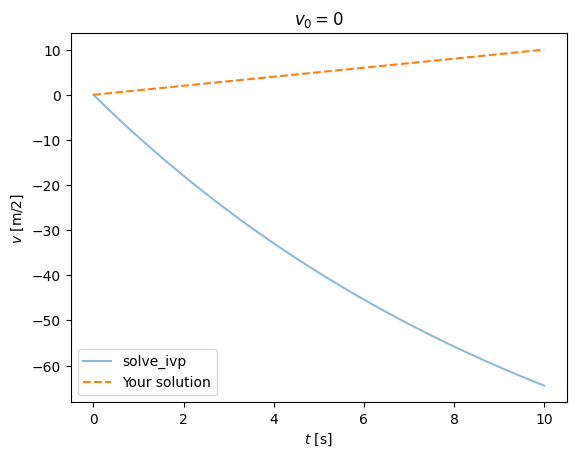
1. Terminal Velocity#

Solve for the motion of a projectile fired vertically with initial velocity \(v(0) = 0\): i.e. dropped from a helicopter. Assume that the drag force is \(F_d = -bv\) so that one has the following differential equation:

\[\begin{gather*} \underbrace{ m \diff{v}{t}}_{ma} = \underbrace{mg - bv}_{F}. \end{gather*}\]

What do you expect the solution to be at large times (i.e. what is the terminal velocity). Check your answer, then check it numerically by comparing with the following code on CoCalc.
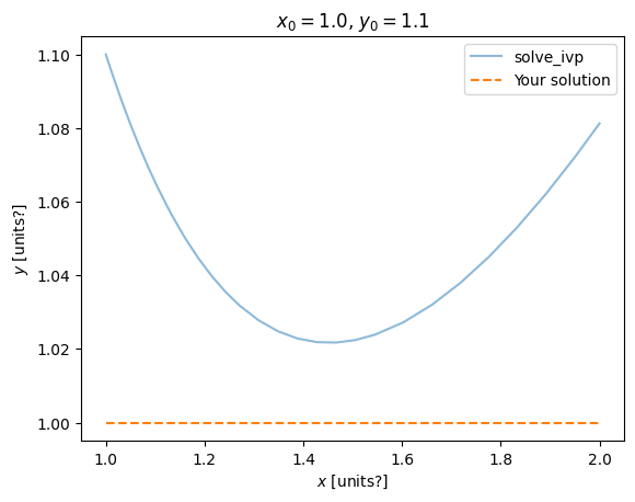
Hide code cell content

%matplotlib inline
import numpy as np, matplotlib.pyplot as plt
from scipy.integrate import solve_ivp

m = 1.1    # Mass in kg
g = -9.81  # Gravitational field in m/s^2
b = 0.1    # Drag coefficient (in what units?)


def compute_dv_dt(t, v):
    return (m*g - b*v)/m


v_0 = 0
t_0, t_1 = 0.0, 10.0
res = solve_ivp(
    compute_dv_dt,
    y0=[v_0],           # solve_ivp needs to be an array or list.
    t_span=(t_0, t_1),
    # The following are optional, but nice to know about
    atol=1e-8,          # Default absolute error goal (when y close to 0)
    rtol=1e-8,          # Default relative error goal (for large |y|)
    max_step=0.1,       # Ensures there are enough points to plot
    method='LSODA',     # More robust that default (but slower)
    dense_output=True,  # Can be used to interpolate
)

t = res.t
v = res.y[0]  # Need to unpack the array returned by solve_ivp

fig, ax = plt.subplots()  # Good practice
ax.plot(t, v, '-', label="solve_ivp", alpha=0.5)
ax.set(xlabel="$t$ [s]", ylabel="$v$ [m/2]",
       title=f"${v_0=}$")


def compute_v(t, v_0=v_0):
    """Put your solution here."""
    return t  #### WRONG

ax.plot(t, compute_v(t), '--', label="Your solution")
ax.legend();
../_images/c2e394ba2bbef9887ee2e101fbb2d286424dbab9be40abbdc5137e3c268e7a82.png

2. An Isobaric ODE.#

Solve the following ODE:

\[\begin{gather*} (x^2 - y^2 e^{y/x})\d{x} + (x^2 + xy)e^{y/x}\d{y} = 0. \end{gather*}\]

Hide code cell content

%matplotlib inline
import numpy as np, matplotlib.pyplot as plt
from scipy.integrate import solve_ivp


def compute_dy_dx(x, y):
    exp_yx = np.exp(y/x)
    return (x**2 - y**2*exp_yx)/(x**2 + x*y)/exp_yx


y_0 = 1.1
x_0, x_1 = 1.0, 2.0
res = solve_ivp(
    compute_dy_dx,
    y0=[y_0],  # solve_ivp needs to be an array or list.
    t_span=(x_0, x_1),
    # The following are optional, but nice to know about
    atol=1e-8,          # Default absolute error goal (when y close to 0)
    rtol=1e-8,          # Default relative error goal (for large |y|)
    max_step=0.1,       # Ensures there are enough points to plot
    method='LSODA',     # More robust that default (but slower)
    dense_output=True,  # Can be used to interpolate
)

x = res.t
y = res.y[0]  # Need to unpack the array returned by solve_ivp

fig, ax = plt.subplots()  # Good practice
ax.plot(x, y, '-', label="solve_ivp", alpha=0.5)
ax.set(xlabel="$x$ [units?]", ylabel="$y$ [units?]", 
       title=f"${x_0=}$, ${y_0=}$")

def compute_y(x, x_0=x_0, y_0=y_0):
    """Put your solution here."""
    return x_0 + 0*x  #### WRONG

ax.plot(x, compute_y(x), '--', label="Your solution")
ax.legend();
../_images/3d0784970744bc72468260375bd5e0a9360d6a929fc276379c85f4f46469034c.png

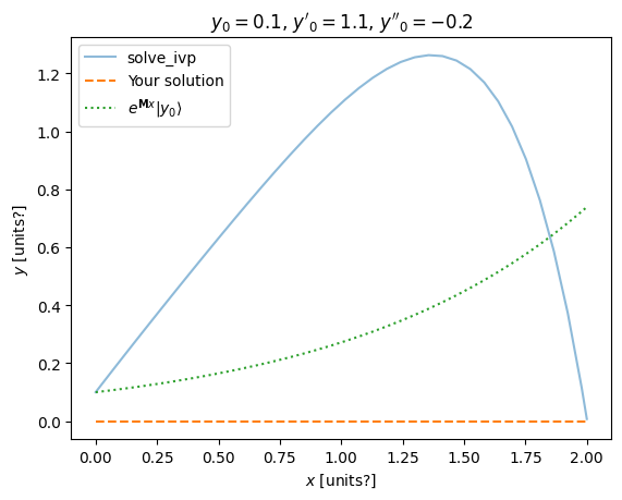
3. Linear Homogeneous ODE with Constant Coefficients#

Find the general solution to the following ODE. Write the solution in forms that are entirely real (i.e., that contain no complex quantities.)

\[\begin{gather*} y''' - 2y'' - y' + 2y = 0. \end{gather*}\]

Explain how to write the equation and your solution as a first-order equation in the form \(\partial_x\ket{y} = \mat{M}\ket{y}\). Check your solution numerically by using solve_ivp and by using expm to exponentiate the matrix.

Hide code cell content

%matplotlib inline
import numpy as np, matplotlib.pyplot as plt
from scipy.integrate import solve_ivp
from scipy.linalg import expm   # Matrix exponential


def compute_dy_dx(x, ys):
    y, dy, ddy = ys
    dddy = 2*ddy + dy - 2*y
    return (dy, ddy, dddy)  # Must be in the same order!


y_0 = 0.1
dy_0 = 1.1
ddy_0 = -0.2

x_0, x_1 = 0.0, 2.0
res = solve_ivp(
    compute_dy_dx,
    y0=[y_0, dy_0, ddy_0], # This is why solve_ivp needs an array or list here
    t_span=(x_0, x_1),
    # The following are optional, but nice to know about
    atol=1e-8,          # Default absolute error goal (when y close to 0)
    rtol=1e-8,          # Default relative error goal (for large |y|)
    max_step=0.1,       # Ensures there are enough points to plot
    method='LSODA',     # More robust that default (but slower)
    dense_output=True,  # Can be used to interpolate
)

x = res.t
y, dy, ddy = res.y      # Unpack the three values returned by solve_ivp

fig, ax = plt.subplots()  # Good practice
ax.plot(x, y, '-', label="solve_ivp", alpha=0.5)
ax.set(xlabel="$x$ [units?]", ylabel="$y$ [units?]", 
       title=f"${y_0=}$, $y'_0={dy_0}$, $y''_0={ddy_0}$")

def compute_y(x, y_0=y_0, dy_0=dy_0, ddy_0=ddy_0):
    """Put your solution here."""
    return x_0 + 0*x  ###### WRONG

ax.plot(x, compute_y(x), '--', label="Your solution")

####### WRONG!  Put the correct matrix here
M = np.array([
    [1, 0, 0],
    [0, 1, 0],
    [0, 0, 1]])

q0 = np.array([y_0, dy_0, ddy_0])

# Here is a simple loop to compute the matrix exponentials.  Not very fast
y = []
for x_ in x:
    q = expm(M*x_) @ q0
    y.append(q[0])

# This is a little trick for better performance.  We make the matrix Mx = M*x
# which has shape (Nx, 3, 3).  expm can then compute the matrix exponentials in
# parallel.

Mx = M[np.newaxis, :, :] * x[:, np.newaxis, np.newaxis]
y_, dy_, ddy = (expm(Mx) @ q0).T   # Transpose needed to flip the indices so we can unpack
assert np.allclose(y, y_)

# Alternatively, you could loop

ax.plot(x, y_, ':', label=r"$e^{\mathbf{M}x}|y_0\rangle$")
ax.legend();
../_images/4a9044b5dd9a920e1cc6f9c34326ad71367adda9719477ac480068abab56bea0.png

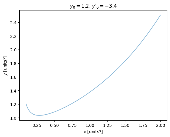
4. Series Solutions 1#

Obtain two series solutions of the confluent hypergeometric equation:

\[\begin{gather*} xy'' + (c-x)y' - ay = 0. \end{gather*}\]

Test your solutions for convergence.

Hide code cell content

%matplotlib inline
import numpy as np, matplotlib.pyplot as plt
from scipy.integrate import solve_ivp

a = 1.0
c = 2.0

def compute_dy_dx(x, ys, a=a, c=c):
    y, dy = ys
    ddy = (a*y - (c-x)*dy)/x
    return (dy, ddy)  # Must be in the same order!


y_0 = 1.2
dy_0 = -3.4
x_0, x_1 = 0.1, 2.0
res = solve_ivp(
    compute_dy_dx,
    y0=[y_0, dy_0], # This is why solve_ivp needs an array or list here
    t_span=(x_0, x_1),
    # The following are optional, but nice to know about
    atol=1e-8,          # Default absolute error goal (when y close to 0)
    rtol=1e-8,          # Default relative error goal (for large |y|)
    max_step=0.1,       # Ensures there are enough points to plot
    method='LSODA',     # More robust that default (but slower)
    dense_output=True,  # Can be used to interpolate
)

x = res.t
y, dy = res.y      # Unpack the three values returned by solve_ivp

fig, ax = plt.subplots()  # Good practice
ax.plot(x, y, '-', label="solve_ivp", alpha=0.5)
ax.set(xlabel="$x$ [units?]", ylabel="$y$ [units?]", 
       title=f"${y_0=}$, $y'_0={dy_0}$")

def compute_y1(x, y_0=y_0, dy_0=dy_0):
    """Put your first series solution here."""
    return x_0 + 0*x  ###### WRONG

def compute_y2(x, y_0=y_0, dy_0=dy_0):
    """Put your second series solution here."""
    return x_0 + 0*x  ###### WRONG
../_images/f5f3f5d6d738640d1138b58dc5ef6e3bf4d4e01d5d39a5e07bad4eb3ae76c903.png

5. Variational Approximation#

Given a self-adjoint operator \(\op{H}\) with a bounded spectrum \(E_0 \leq E_n\), use the fact that the eigenfunctions \(\op{H}\ket{n} = \ket{n}E_n\) form a complete basis to prove the variation method or variational theorem:

\[\begin{gather*} E_0 \leq \braket{\psi|\op{H}|\psi}. \end{gather*}\]

I.e., we can find an upper bound on the lowest eigenvalue \(E_0\) by guessing a trial function \(\ket{\psi}\) and minimizing over the parameters.

Apply this to provide a bound for the ground state of hydrogen by guessing a form for the radial wavefunction \(u(r)\) for \(r\in[0, \infty]\) which goes to zero at \(r=0\) and \(r=\infty\).

\[\begin{gather*} -u''(r) - \frac{u(r)}{r} = Eu(r). \end{gather*}\]

I.e., guess something reasonable for \(u(r)\) with one or more parameters, and minimize

\[\begin{gather*} E_0 \leq \frac{\braket{u|\op{H}|u}}{\braket{u|u}} = \frac{\int_0^{\infty}\d{r}\;\left(\abs{u'(r)}^2 - \frac{\abs{u(r)}^2}{r}\right)} {\int_0^{\infty}\d{r}\;\abs{u(r)}^2}. \end{gather*}\]

Hint.

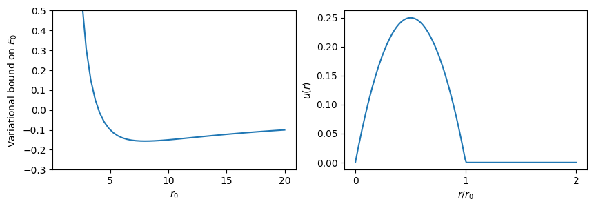
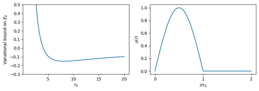
If you don’t have a better idea, you could try a parabola:

\[\begin{gather*} u(r) = \begin{cases} r(r_0-r) & r < r_0,\\ 0 & r \geq r_0. \end{cases} \end{gather*}\]

The numerical results are below for you to check your work.

Hide code cell source

from scipy.integrate import quad

def u(r, r0, d=0):
    """Return the radial wavefunction or its derivative (if d=1)"""
    if d == 0:
        return r*(r0-r)
    else:
        return r0 - 2*r

def uHu(r, *v):
    """Return the integrand in the numerator."""
    return abs(u(r, *v, d=1))**2 - abs(u(r, *v))**2/r

def u2(r, *v):
    """Return the square of the radial function for normalization."""
    return abs(u(r, *v))**2

def get_variational_bound(r0):
    return (quad(uHu, 0, r0, args=(r0,))[0] /
            quad(u2, 0, r0, args=(r0,))[0])

rs = np.linspace(1, 20.0, 50)
Es = [get_variational_bound(r0) for r0 in rs]
fig, axs = plt.subplots(1, 2, figsize=(10, 3))
ax = axs[0]
ax.plot(rs, Es)
ax.set(ylim=(-0.3,0.5), xlabel="$r_0$", ylabel="Variational bound on $E_0$");
ax = axs[1]
r = np.linspace(0, 2, 200)
ax.plot(r, np.where(r<1.0, u(r, r0=1), 0))
ax.set(xlabel="$r/r_0$", ylabel="$u(r)$", xticks=[0, 1, 2]);
print(f"E ≤ {min(Es):.5g}")
E ≤ -0.15625
../_images/f58e71e610ac9c97d0531b9c85865e5b2089e5865ba3fccca8d5eda27c20f8ed.png

Hide code cell content

from scipy.integrate import quad

def u(r, r0, d=0):
    """Return the radial wavefunction or its derivative (if d=1)"""
    if d == 0:
        return np.sin(np.pi * r/r0)
    else:
        return np.pi/r0 * np.cos(np.pi * r/r0)

def uHu(r, *v):
    """Return the integrand in the numerator."""
    return abs(u(r, *v, d=1))**2 - abs(u(r, *v))**2/r

def u2(r, *v):
    """Return the square of the radial function for normalization."""
    return abs(u(r, *v))**2

def get_variational_bound(r0):
    return (quad(uHu, 0, r0, args=(r0,))[0] /
            quad(u2, 0, r0, args=(r0,))[0])

rs = np.linspace(1, 20.0, 50)
Es = [get_variational_bound(r0) for r0 in rs]
fig, axs = plt.subplots(1, 2, figsize=(10, 3))
ax = axs[0]
ax.plot(rs, Es)
ax.set(ylim=(-0.3,0.5), xlabel="$r_0$", ylabel="Variational bound on $E_0$");
ax = axs[1]
r = np.linspace(0, 2, 200)
ax.plot(r, np.where(r<1.0, u(r, r0=1), 0))
ax.set(xlabel="$r/r_0$", ylabel="$u(r)$", xticks=[0, 1, 2]);
print(f"E ≤ {min(Es):.5g}")
E ≤ -0.15048
../_images/a7cd42a6b20143274fb659d1dec28c82746b50d8ece4a3e2e281a01a54719f4a.png

Hide code cell content

from scipy.integrate import quad

def u(r, r0, d=0):
    """Return the radial wavefunction or its derivative (if d=1)"""
    if d == 0:
        return 0.5 - abs(r/r0-0.5)
    else:
        return  - np.sign(r/r0-0.5)/r0

def uHu(r, *v):
    """Return the integrand in the numerator."""
    return abs(u(r, *v, d=1))**2 - abs(u(r, *v))**2/r

def u2(r, *v):
    """Return the square of the radial function for normalization."""
    return abs(u(r, *v))**2

def get_variational_bound(r0):
    return (quad(uHu, 0, r0, args=(r0,))[0] /
            quad(u2, 0, r0, args=(r0,))[0])

rs = np.linspace(1, 20.0, 50)
Es = [get_variational_bound(r0) for r0 in rs]
fig, axs = plt.subplots(1, 2, figsize=(10, 3))
ax = axs[0]
ax.plot(rs, Es)
ax.set(ylim=(-0.3,0.5), xlabel="$r_0$", ylabel="Variational bound on $E_0$");
ax = axs[1]
r = np.linspace(0, 2, 200)
ax.plot(r, np.where(r<1.0, u(r, r0=1), 0))
ax.set(xlabel="$r/r_0$", ylabel="$u(r)$", xticks=[0, 1, 2]);
print(f"E ≤ {min(Es):.5g}")
E ≤ -0.11192
../_images/abd9722aab86cf6f02305de7998b6380b2cce069141bf648ad0d21afb0e89e29.png

Note

A few of notes.

  1. We have integrated by parts here to write

    \[\begin{gather*} \int_0^{\infty}\d{r}\;\Bigl(-u^*(r)u''(r)\Bigr) = \int_0^{\infty}\d{r}\;\abs{u'(r)}^2. \end{gather*}\]

    The boundary terms vanish since \(u(0) = u(\infty) = 0\).

  2. We have chosen units so that \(\hbar^2/2\mu = e^2/4\pi\epsilon_0 = 1\) where \(\mu = m_em_p/(m_e+m_p)\) is the reduced mass. This means that your energy will be expressed in units of the following:

    \[\begin{gather*} 1 = \overbrace{\underbrace{ \frac{\hbar^2}{2\mu}\frac{4\pi\epsilon_0}{e^2} }_{\text{distance}}}^{\approx 0.2647\text{Å}\atop \approx 2.647\times 10^{-11}\text{m}} = \overbrace{\underbrace{ \frac{2\mu}{\hbar^2}\left(\frac{e^2}{4\pi\epsilon_0}\right)^2 }_{\text{energy}}}^{\approx 54.38\text{eV} \atop \approx 8.715\times 10^{-18}\text{J}} \end{gather*}\]

    Thus, multiply your numerical bound by \(54.38\,\)eV to check.

  3. This equation comes from noting that the ground state has zero angular momentum \(l=0\), so the wavefunction can be written

    \[\begin{gather*} \psi(\vect{x}) = Y^{0}_{0}(\theta, \phi)\psi_0(r), \qquad \psi_0(r) = \frac{u_0(r)}{r}, \end{gather*}\]

    where \(\vect{x}\) is the vector separating the electron and proton, and \(\psi_{0}(r) = ru_0(r)\) is the radial wavefunction which satisfies:

    \[\begin{gather*} \left(-\frac{1}{r^2}\pdiff{}{r}\left(r^2 \pdiff{}{r}\right) - \frac{1}{r}\right)\psi_0(r) = E_0\psi_0(r) \end{gather*}\]

    after setting our units.

  4. Note that, in spherical coordinates, we should integrate with the metric \(4\pi r^2 \d{r}\). The normalization would thus be:

    \[\begin{gather*} 1 = \int_0^{\infty} 4\pi r^2\d{r}\; \abs{\psi_0(r)}^2 = \int_0^{\infty} 4\pi r^2\d{r}\; \frac{\abs{u(r)}^2}{r^2} = 4\pi \int_0^{\infty} \d{r}\; \abs{u(r)}^2. \end{gather*}\]

    The factor of \(4\pi\) will cancel from the numerator and denominator in the variational bound, and so we are able to neglect it.

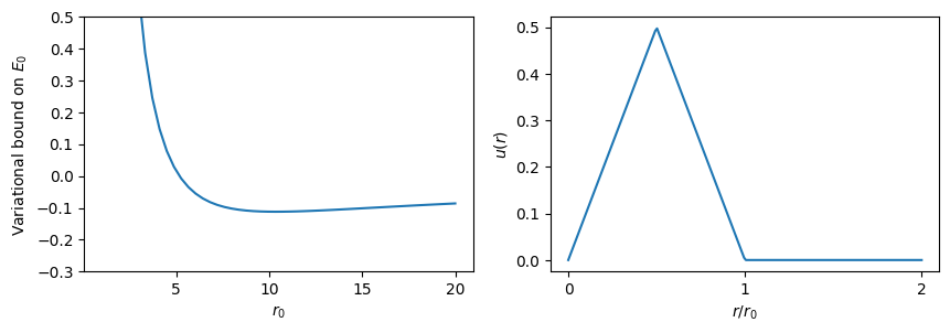
  5. You might consider simpler trial functions, but be sure they do not have discontinuities. For example, the function

    \[\begin{gather*} u(r) = \begin{cases} r & r < r_0\\ 0 & r > r_0 \end{cases} \end{gather*}\]

    seems to work, and gives a nice “bound” if you make a mistake and forget the fact that \(u'(r)\) has a delta function at \(r=r_0\). If you include this delta function, you get the rather unhelpful bound \(E\leq\infty\).