Show code cell content

Hide code cell content

import mmf_setup;mmf_setup.nbinit()
import logging;logging.getLogger('matplotlib').setLevel(logging.CRITICAL)
%matplotlib inline
import numpy as np, matplotlib.pyplot as plt

$\newcommand{\vect}[1]{\mathbf{#1}} \newcommand{\uvect}[1]{\hat{#1}} \newcommand{\abs}[1]{\lvert#1\rvert} \newcommand{\norm}[1]{\lVert#1\rVert} \newcommand{\I}{\mathrm{i}} \newcommand{\ket}[1]{\left|#1\right\rangle} \newcommand{\bra}[1]{\left\langle#1\right|} \newcommand{\braket}[1]{\langle#1\rangle} \newcommand{\Braket}[1]{\left\langle#1\right\rangle} \newcommand{\op}[1]{\mathbf{#1}} \newcommand{\mat}[1]{\mathbf{#1}} \newcommand{\d}{\mathrm{d}} \newcommand{\D}[1]{\mathcal{D}[#1]\;} \newcommand{\pdiff}[3][]{\frac{\partial^{#1} #2}{\partial {#3}^{#1}}} \newcommand{\diff}[3][]{\frac{\d^{#1} #2}{\d {#3}^{#1}}} \newcommand{\ddiff}[3][]{\frac{\delta^{#1} #2}{\delta {#3}^{#1}}} \newcommand{\floor}[1]{\left\lfloor#1\right\rfloor} \newcommand{\ceil}[1]{\left\lceil#1\right\rceil} % The following allows KaTeX to render these for significantly improved % performance on CoCalc. \newcommand{\DeclareMathOperator}[2]{\newcommand{#1}{#2}} \DeclareMathOperator{\Tr}{Tr} \DeclareMathOperator{\erf}{erf} \DeclareMathOperator{\erfi}{erfi} \DeclareMathOperator{\sech}{sech} \DeclareMathOperator{\sn}{sn} \DeclareMathOperator{\cn}{cn} \DeclareMathOperator{\dn}{dn} \DeclareMathOperator{\sgn}{sgn} \DeclareMathOperator{\order}{O} \DeclareMathOperator{\diag}{diag} % \newcommand{\mylabel}[1]{\label{#1}\tag{#1}} \newcommand{\degree}{\circ}$

This cell adds /home/docs/checkouts/readthedocs.org/user_builds/physics-571-math-methods/checkouts/latest/src to your path, and contains some definitions for equations and some CSS for styling the notebook. If things look a bit strange, please try the following:

• Choose "Trust Notebook" from the "File" menu.
• Re-execute this cell.
• Reload the notebook.

Assignment 6: Orthonormal Bases

Due Mon 13 Oct 2025 at the start of class

For this assignment, I recommend you use Dirac’s braket notation as much as possible.

1. Uniqueness

Suppose a function \(f(x)\) is expanded in series of orthonormal functions

\[\begin{gather*} f(x) = \sum_{n=0}^{\infty}a_n\phi_n(x). \end{gather*}\]

Show that the series expansion is unique for a given set of basis functions \(\phi_n(x)\) that form a complete basis for an infinite-dimensional Hilbert space.

2. Changing Bases

The explicit form of a function \(f\) is not known, but the coefficients \(a_n\) of its expansion in an orthonormal set \(\phi_n\) is available. Assuming that the \(\phi_n\) and the members of another orthonormal set, \(\chi_n\), are available, use Dirac notation to obtain a formula for the coefficients for the expansion of \(f\) in the \(\chi_n\) set.

3. Gram-Schmidt

Sometimes these shifted Legendre polynomials are are denoted \(P^*_n(x)\) in contrast to \(P_n(x)\), which are orthogonal over \([-1, 1]\). The “\(*\)” does not mean complex conjugation in this case.

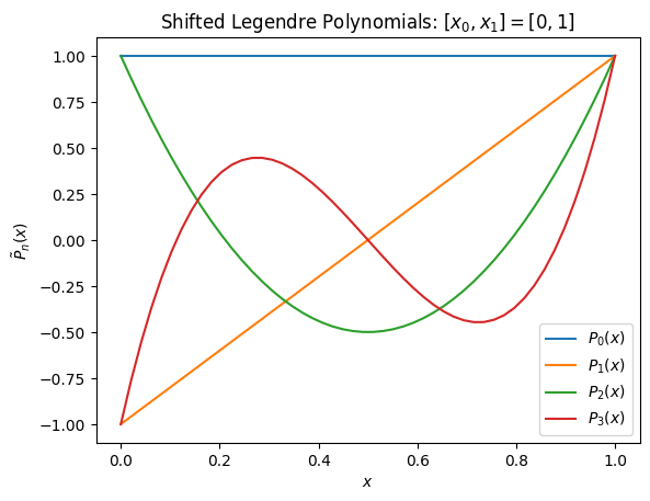
Following the Gram-Schmidt procedure, construct the first three polynomials \(\tilde{P}_n(x)\) orthogonal (unit weighting factor) over the range \([0, 1]\) from the set \([1, x, x^2, \dots]\). Scale so that \(\tilde{P}_n(1)=1\). These are the first three shifted Legendre polynomials, shifted to be orthogonal over the interval \([0, 1]\) instead of \([-1, 1]\).

4. A Small Hilbert Space (Arfken 5.3.3)

Note: this 3-dimensional Hilbert space \(\mathcal{H}\) is a subset of the functions from \(\mathbb{R}^3\rightarrow \mathbb{R}\): \(\psi(x_1, x_2, x_3)\) . The form of the inner product is not specified: the idea is to assume that it has some form, but to just use the defined inner product. If you insist on a concrete representation, what about

\[\begin{gather*} \braket{f|g} = \frac{3}{8}\int_{-1}^{1}\int_{-1}^{1}\int_{-1}^{1}fg\;\d{x_1}\d{x_2}\d{x_3}. \end{gather*}\]

Note that the operators \(A_1\) and \(A_2\) keep vectors from \(\mathcal{H}\) in \(\mathcal{H}\): e.g., they do not produce things like \(x_1^2\) or a constant \(c\) which are not expressible in the basis.

Consider a Hilbert space spanned by three functions \(\phi_1 = x_1\), \(\phi_2 = x_2\), \(\phi_3 = x_3\), and an inner product defined by \(\braket{x_\nu|x_\mu} = \delta_{\nu\mu}\).

1. Form the \(3\times 3\) matrix for each of the following operators:

   \[\begin{gather*} {A}_1 = \sum_{i=1}^{3} x_{i}\left(\pdiff{}{x_i}\right), \qquad {A}_2 = x_1\left(\pdiff{}{x_2}\right) - x_2\left(\pdiff{}{x_1}\right). \end{gather*}\]

2. Form the column vector representing \(\psi = x_1 - 2x_2 + 3x_3\).

3. Form the matrix equation corresponding to \(\chi = ({A}_1 - {A}_2)\psi\) and verify that the matrix equation reproduces the results obtained by direct application of \({A}_1 - {A}_2\) to \(\psi\).

5. Check your results.

Check your results with the following code (or similar). Note that NumPy as many tools such as orthogonal polynomials for you to use in np.polynomial. I use this to provide skeletons and check that the testing code works, and to show you how to use these if you need them.

Gram-Schmidt: Shifted Legendre Polynomials

Check your expressions for \(\tilde{P}_{n}(x)\) with the following code which defines a braket function to check the orthogonality.

\[\begin{gather*} \braket{f|g} = \int_{a}^{b} f^*(x)g(x)\d{x}. \end{gather*}\]

This code is easily generalized to other intervals or to include a weighting function \(w(x)\). You should start thinking about how you might compute these. We will return to this when we return to Chapter 12.1 in [].

#:tags: [hide-input]
%matplotlib inline
import numpy as np, matplotlib.pyplot as plt
from numpy.polynomial.legendre import Legendre
from scipy.integrate import quad

x0, x1 = [0, 1]  # Interval

def braket(f, g, x0=x0, x1=x1):
    """Return ⟨f|g⟩."""
    return quad(lambda x:np.conj(f(x))*g(x), x0, x1)[0]


###### Put your functions here
def P(x, n=0, x0=x0, x1=x1):
    """Return the nth shifted Legendre polynomial."""
    if n == 0:
        return np.ones_like(x)  # Make it an array
    elif n == 1:
        # Put your expressions here and uncomment
        # return x
        P1 = Legendre([0, 1], domain=[x0, x1])  # CHEATING!
        return P1(x)
    elif n == 2:
        # Put your expressions here and uncomment
        # return x**2
        P2 = Legendre([0, 0, 1], domain=[x0, x1])  # CHEATING!
        return P2(x)
    else:
        # CHEATING!
        c = np.zeros(n+1)
        c[-1] = 1
        P = Legendre(c, domain=[x0, x1])
        return P(x)

# Check and plot $N$ polynomials
N = 4

fig, ax = plt.subplots()  # Good practice
x = np.linspace(x0, x1)
for n in range(N):
    ax.plot(x, P(x, n=n), label=f"$P_{n}(x)$")
ax.set(xlabel="$x$", ylabel=r"$\tilde{P}_n(x)$", 
       title=f"Shifted Legendre Polynomials: $[x_0,x_1]=[{x0}, {x1}]$")
ax.legend()

braket_mn = np.zeros((N, N))
for n in range(N):
    for m in range(N):
        braket_mn[m, n] = braket(lambda x: P(x, m), lambda x: P(x, n))

print("Here are the overlaps and diagonals.  Use this to help you debug if")
print("the following checks fail.")
print("⟨Pm|Pn⟩ = ")
print(braket_mn)
print(f"⟨Pn|Pn⟩ = {np.diag(braket_mn)}")

# Check that it is diagonal (orthogonality)
assert np.allclose(braket_mn, np.diag(np.diag(braket_mn)))

# Check normalization as specified in the problem
assert np.allclose([P(1, n) for n in range(N)], 1)

Here are the overlaps and diagonals.  Use this to help you debug if
the following checks fail.
⟨Pm|Pn⟩ = 
[[1.00000000e+00 3.51635587e-18 4.16333634e-17 6.65397041e-18]
 [3.51635587e-18 3.33333333e-01 5.08516314e-18 8.32667268e-17]
 [4.16333634e-17 5.08516314e-18 2.00000000e-01 1.97446957e-18]
 [6.65397041e-18 8.32667268e-17 1.97446957e-18 1.42857143e-01]]
⟨Pn|Pn⟩ = [1.         0.33333333 0.2        0.14285714]

Expanding Functions in Bases

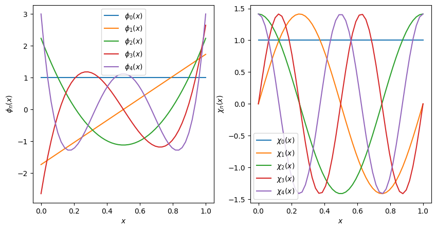
Now that we have code to compute \(\tilde{P}_n(x)\) we can define an orthonormal basis to demonstrate the expansion of functions. First we must normalize them. We do this numerically with the braket function we defined above

\[\begin{gather*} \phi_n(x) = \frac{\tilde{P}_{n(x)}}{\sqrt{\braket{P_n|P_n}}}. \end{gather*}\]

To demonstrate the change of basis, we define another set of orthonormal basis functions which we will discuss in Fourier Series in Chapter 19 of [Arfken et al., 2013]:

\[\begin{gather*} S_n(x) = \sin(2\pi n x), \qquad C_n = \cos(2\pi n x)\\ X_n = [C_0, S_1, C_1, S_2, C_2, \dots],\\ \chi_n(x) = \frac{X_{n}(x)}{\sqrt{\braket{X_n|X_n}}}. \end{gather*}\]

%matplotlib inline
import numpy as np, matplotlib.pyplot as plt
from numpy.polynomial.legendre import Legendre
from scipy.integrate import quad

x0, x1 = [0, 1]  # Interval

def braket(f, g, x0=x0, x1=x1):
    """Return ⟨f|g⟩."""
    return quad(lambda x:np.conj(f(x))*g(x), x0, x1)[0]


def get_phi(n, x0=x0, x1=x1):
    """Return the nth basis function."""
    c = np.zeros(n+1)
    c[-1] = 1
    P = Legendre(c, domain=[x0, x1])

    # P is a special function object that you can scale...
    phi = P / np.sqrt(braket(P, P))
    return phi


def get_chi(n, x0=x0, x1=x1):
    """Return the nth basis function."""
    if n % 2 == 0:
        # n is even, use cosine
        m = n//2
        X = lambda x: np.cos(2*np.pi*m * x)
    else:
        # N is odd, use cosine
        m = (n+1)//2
        X = lambda x: np.sin(2*np.pi*m * x)

    # Normalize. We can't scale X like we did P, so we define a new function 
    tmp = np.sqrt(braket(X, X)) 
    chi = lambda x: X(x) / tmp
    return chi


x = np.linspace(x0, x1)
fig, axs = plt.subplots(1, 2, figsize=(10,5))
N = 5
ax_phi = axs[0]
ax_chi = axs[1]
for n in range(N):
    ax_phi.plot(x, get_phi(n)(x), label=rf"$\phi_{{{n}}}(x)$")
    ax_chi.plot(x, get_chi(n)(x), label=rf"$\chi_{{{n}}}(x)$")

ax_phi.set(xlabel="$x$", ylabel=r"$\phi_n(x)$")
ax_chi.set(xlabel="$x$", ylabel=r"$\chi_n(x)$")
for ax in axs:
    ax.legend()

# Check orthonormality
phi_mn = np.array(
    [[braket(get_phi(m), get_phi(n)) for n in range(N)]
     for m in range(N)])
chi_mn = np.array(
    [[braket(get_chi(m), get_chi(n)) for n in range(N)]
     for m in range(N)])
assert np.allclose(phi_mn, np.eye(N))
assert np.allclose(chi_mn, np.eye(N))

Use these basis functions and braket to test your expressions for problems 1. and 2. Specifically:

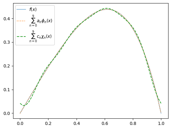
1. Compute the coefficients \(a_n\) for \(f(x) = x(1-x)e^x\):

   \[\begin{gather*} f(x) = x(1-x)e^{x} \approx \sum_{n=0}^{N-1} a_n \phi_n(x) \end{gather*}\]

2. Using only these \(a_n\), use your expression from problem 2. to compute the coefficients \(c_n\) such that

   \[\begin{gather*} f(x) = x(1-x)e^{x}e^{x} \approx \sum_{n=0}^{N-1} c_n\chi_n(x). \end{gather*}\]

3. Use the following code to plot how the maximum error scales with the number of terms \(N\).

def f(x):
    return x*(1-x)*np.exp(x)
    return np.exp(x)
    return np.exp(np.sin(2*np.pi*x))
    return np.exp(-1/x/(1-x))
    
N = 10
a = np.zeros(N)  # Arrays for the coefficients
c = np.zeros(N)  # Arrays for the coefficients
phi = [get_phi(n) for n in range(N)]
chi = [get_chi(n) for n in range(N)]

# First play and figure out how to compute a[n]
for n in range(N):
    a[n] = braket(phi[n], f)
    c[n] = braket(chi[n], f)  # Direct expansion... don't use here

## Put your answer to problem 2. in here.  Consider np.linalg.solve(A, b)
## which solve A@x = b.

A = np.zeros((N, N))
for m in range(N):
    for n in range(N):
        A[m, n] = 0
#c = np.linalg.solve(A, a)

# Check
fig, ax = plt.subplots()
x = np.linspace(x0, x1)
ax.plot(x, f(x), label="$f(x)$", alpha=0.5)

f_phi = sum(a[n]*phi[n](x) for n in range(N))
ax.plot(x, f_phi, ':', label=rf"$\sum_{{n=0}}^{{{N-1}}} a_n\phi_n(x)$")

f_chi = sum(c[n]*chi[n](x) for n in range(N))
ax.plot(x, f_chi, '--', label=rf"$\sum_{{n=0}}^{{{N-1}}} c_n\chi_n(x)$")

ax.legend();

Now we repeat everything, but in a function so we can plot the maximum error as a function of \(N\):

def get_approx(N, get_phi=get_phi, f=f, x=x):
    phi = [get_phi(n) for n in range(N)]
    a = [braket(phi[n], f) for n in range(N)]
    f_phi = sum(a[n]*phi[n](x) for n in range(N)) 
    return f_phi

Ns = 2**np.arange(6)
max_errs_phi = [max(abs(get_approx(N, get_phi=get_phi) - f(x))) for N in Ns]
max_errs_chi = [max(abs(get_approx(N, get_phi=get_chi) - f(x))) for N in Ns]
mean_errs_phi = [np.mean(abs(get_approx(N, get_phi=get_phi) - f(x))) for N in Ns]
mean_errs_chi = [np.mean(abs(get_approx(N, get_phi=get_chi) - f(x))) for N in Ns]
fig, axs = plt.subplots(1, 2, figsize=(10,4))
for N in Ns:
    axs[0].plot(x, get_approx(N, get_phi=get_phi), label=f"$N={int(N)}$")
    axs[1].plot(x, get_approx(N, get_phi=get_chi), label=f"$N={int(N)}$")

for ax in axs:
    ax.plot(x, f(x), '-k')
    ax.legend()

fig, ax = plt.subplots(figsize=(10,4))
ax.loglog(Ns, max_errs_phi, '-C0x', label=r"$\phi_n$ (shifted Legendre) max err")
ax.loglog(Ns, mean_errs_phi, ':C0x', label=r"$\phi_n$ (shifted Legendre) mean err")
ax.loglog(Ns, max_errs_chi, '-C1o', label=r"$\chi_n$ (Fourier) max err")
ax.loglog(Ns, mean_errs_chi, ':C1o', label=r"$\chi_n$ (Fourier) mean err")
ax.set_xscale('log', base=2)
ax.set(xlabel="$N$", ylabel="Absolute Error")
ax.legend();

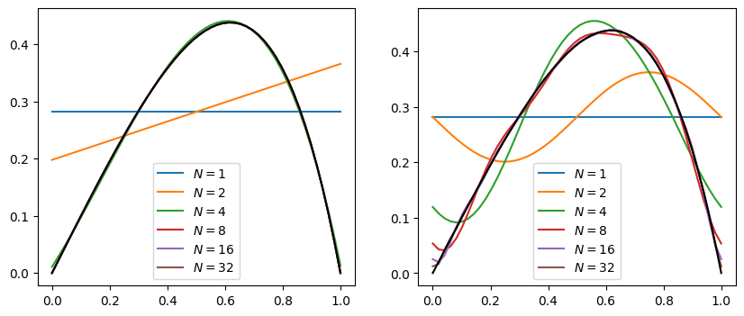
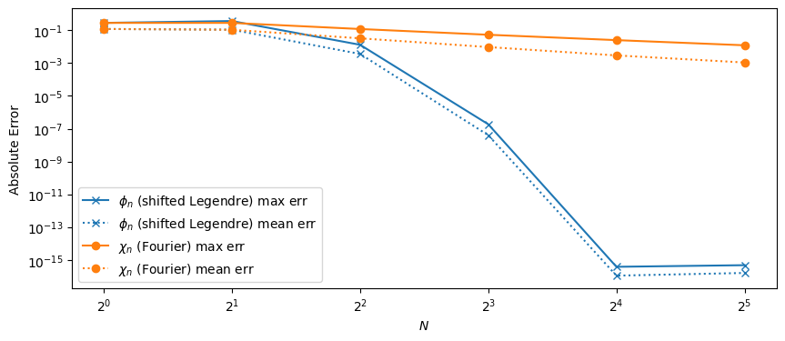
Notice that the Fourier basis does not converge very well, partly due to the Gibbs phenomena, but the shifted Legendre basis works extremely well. Can you give a (quantitative) argument why? Try with different functions \(f(x)\). Can you find examples where the Fourier basis works much better than the shifted Legendre basis?

Midterm Exam Question: Harmonic Oscillator

To recover units, multiply by the appropriate factor of \(1\):

\[\begin{gather*} 1 = \underbrace{\hbar\omega}_{\text{energy}} = \underbrace{\sqrt{\frac{\hbar}{m\omega}}}_{\text{distance}} = \underbrace{\sqrt{m\hbar \omega}}_{\text{momentum}} = \dots \end{gather*}\]

etc.

Here we use the Hermite polynomials to look at the wavefunction from the last question of the Midterm I Exam. Here the eigenstates are expressed in terms of the Hermite polynomials

\[\begin{gather*} \psi_n(x) = \braket{x|n} \propto e^{-x^2/2}H_n(x) \end{gather*}\]

where we have chosen units such that \(\hbar = m = \omega = 1\).

To compute the momentum acting on these states, we will need to take the derivative:

\[\begin{gather*} \psi_n'(x) \propto \bigl(H_n'(x) - xH_n(x)\Bigr)e^{-x^2/2} \end{gather*}\]

import numpy as np
from numpy.polynomial.hermite import Hermite, hermmulx
from scipy.integrate import quad

# These are all 1.
hbar = m = w = 1.0  # Units
a0 = np.sqrt(hbar/m/w)  # Length unit (oscillator length)
E0 = hbar*w  # Energy unit

def braket(f, g, complex=False):
    # We must include the Gaussian weight here
    return  quad(lambda x: np.conj(f(x))*g(x)*np.exp(-x**2), 
                 -np.inf, np.inf, 
                 complex_func=complex)[0]
    
def get_H(n):
    """Return the normalized basis polynomial (no gaussian)."""
    c = np.zeros(n+1)
    c[-1] = 1
    H = Hermite(c)
    c[-1] = 1/np.sqrt(braket(H, H))
    return Hermite(c)

def op_X(psi):
    """Act with x on psi (assumes psi is a Hermite polynomial."""
    return Hermite(hermmulx(psi.coef))

def op_iP(psi):
    """Act with i*P on psi (assumes psi is a Hermite polynomial."""
    return hbar*(psi.deriv() - op_X(psi))
    
N = 5
H = [get_H(m) for m in range(N)]
braket_mn = np.zeros((N, N))
for n in range(N):
    for m in range(N):
        braket_mn[m, n] = braket(H[m], H[n])

# Check that it is diagonal (orthogonality)
assert np.allclose(braket_mn, np.eye(N))

x_mn = np.zeros((N, N))
ip_mn = np.zeros((N, N))
for n in range(N):
    for m in range(N):
        x_mn[m, n] = braket(H[m], op_X(H[n]))
        ip_mn[m, n] = braket(H[m], op_iP(H[n]))

print("2⟨m|x|n⟩^2 = ")
print(np.round(2*np.sign(x_mn)*x_mn**2, 8))
print("2⟨m|ip|n⟩^2 = ")
print(np.round(2*np.sign(ip_mn)*ip_mn**2, 8))

X = x_mn
P = ip_mn/1j

ihbar = X@P - P@X
assert np.allclose(ihbar.real, 0)
print("[X,P]/i = ") 
print(np.round((ihbar/1j).real, 8))

2⟨m|x|n⟩^2 = 
[[ 0.  1.  0. -0.  0.]
 [ 1.  0.  2.  0. -0.]
 [ 0.  2.  0.  3.  0.]
 [-0.  0.  3.  0.  4.]
 [ 0.  0.  0.  4.  0.]]
2⟨m|ip|n⟩^2 = 
[[ 0.  1.  0.  0.  0.]
 [-1.  0.  2.  0.  0.]
 [ 0. -2.  0.  3.  0.]
 [ 0.  0. -3.  0.  4.]
 [ 0. -0.  0. -4.  0.]]
[X,P]/i = 
[[ 1.  0. -0.  0.  0.]
 [ 0.  1.  0.  0.  0.]
 [-0.  0.  1.  0.  0.]
 [ 0.  0.  0.  1.  0.]
 [-0.  0. -0.  0. -4.]]

Note that this demonstrates an interesting point. From quantum mechanics, we expect the commutation relationship

\[\begin{gather*} [\op{x}, \op{p}] = \I\hbar. \end{gather*}\]

However, as you proved in an earlier assignment, the trace of a commutator of matrices is always zero \(\Tr[\mat{A}, \mat{B}] = 0\). This result need not hold for infinite dimensional systems, but it is interesting to see how this happens in finite-dimensional approximations. We see here that the trace of the commutator is indeed zero, but that the correction term occurs at the boundary (the \(-4\) above), which gets pushed out to “infinity” as we include more and more states.

We see from these manipulations that the position and momentum operators have the following form in the harmonic oscillator basis:

\[\begin{gather*} \braket{m|\op{x}|n} = \sqrt{\frac{\hbar}{2m\omega}} \begin{pmatrix} 0 & 1\\ 1 & 0 & \sqrt{2}\\ & \sqrt{2} & 0 & \sqrt{3}\\ & & \sqrt{3} & 0 & \ddots\\ & & & \ddots & \ddots \end{pmatrix},\\ \braket{m|\op{p}|n} = \I\sqrt{\frac{\hbar m \omega}{2}} \begin{pmatrix} 0 & 1\\ -1 & 0 & \sqrt{2}\\ & -\sqrt{2} & 0 & \sqrt{3}\\ & & -\sqrt{3} & 0 & \ddots\\ & & & \ddots & \ddots \end{pmatrix}. \end{gather*}\]

These were codified on the midterm as

\[\begin{gather*} \op{x}\ket{n} = \sqrt{\frac{\hbar}{2m\omega}}\Big(\ket{n+1}\sqrt{n+1} + \ket{n-1}\sqrt{n}\Bigr),\\ \op{p}\ket{n} = \I\sqrt{\frac{\hbar m\omega}{2}}\Big(\ket{n+1}\sqrt{n+1} - \ket{n-1}\sqrt{n}\Bigr). \end{gather*}\]

Make sure you understand the relationship between these two representations.

We can now look at the wavefunction corresponding to the state \(\ket{\psi} = (\ket{0} + \I \ket{1})/\sqrt{2}\):

c = 1j
c /= abs(c)
H = (get_H(0) + c*get_H(1))/np.sqrt(2)
x = np.linspace(-4, 4)
fig, ax = plt.subplots()
psi_x = H(x) * np.exp(-x**2/2)
ax.plot(x, psi_x.real, '--', label=r"$\mathrm{Re} \psi$")
ax.plot(x, psi_x.imag, ':', label=r"$\mathrm{Im} \psi$")
ax.plot(x, abs(psi_x)**2, '-k', label=r"$|\psi|^2$")
ax.set(xlabel=r"$x/\sqrt{\hbar/m\omega}$")
ax.legend();

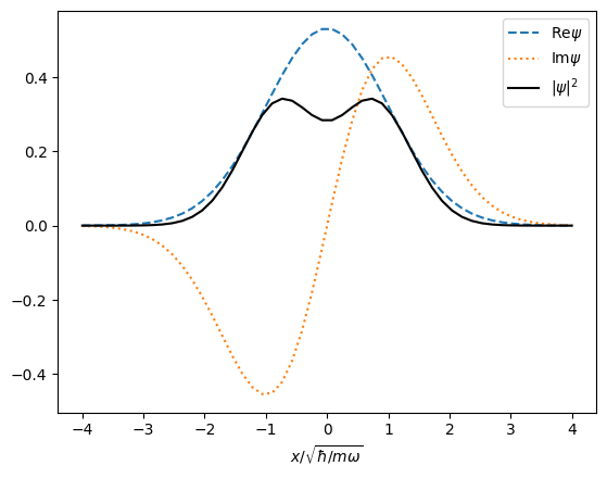
Play with this a bit: note that the state does indeed have zero expectation for \(\braket{\op{x}} = 0\), but only if \(c=\I\). If \(c\) has any real part, there is interference.

For good measure, here is an animation of the time-dependence of the state. Make sure you understand the code get_psi(t):

E0, E1 = 1/2, 3/2  # Energy eigenvalues in units of hbar*w

psi0 = get_H(0)(x)*np.exp(-x**2/2)
psi1 = get_H(1)(x)*np.exp(-x**2/2)

def get_psi(t, x=x):
    """Return psi at time t."""
    return (np.exp(E0*t/1j) * psi0 + 1j*np.exp(E1*t/1j) * psi1)/np.sqrt(2)

Here is a movie. Note that the state is not a stationary state: it starts with non-zero average momentum and oscillates in the trap.

Show code cell source

Hide code cell source

# Make a movie
from matplotlib.animation import FuncAnimation
from IPython.display import HTML, display

fig, ax = plt.subplots()
psi_x = get_psi(t=0, x=x)
l_re, = ax.plot(x, psi_x.real, '--', label=r"$\mathrm{Re} \psi$")
l_im, = ax.plot(x, psi_x.imag, ':', label=r"$\mathrm{Im} \psi$")
l_p2, = ax.plot(x, abs(psi_x)**2, '-k', label=r"$|\psi|^2$")
ax.set(xlabel=r"$x/\sqrt{\hbar/m\omega}$")
ax.legend();

def init():
    ax.set(ylim=(-0.5, 0.75))
    return l_re, l_im, l_p2

def update(t):
    psi_x = get_psi(t=t, x=x)
    l_re.set_data(x, psi_x.real)
    l_im.set_data(x, psi_x.imag)
    l_p2.set_data(x, abs(psi_x)**2)
    return l_re, l_im, l_p2

ani = FuncAnimation(
    fig, update, frames=np.linspace(0, 4*np.pi, 2*128), init_func=init, blit=True)

display(HTML(ani.to_jshtml(fps=100)))
plt.close('all')

Once Loop Reflect