Traffic Flow

Traffic Flow#

The continuum description of traffic flow on a road (1D) can be expressed in terms of the traffic density \(n(x,t)\) and velocity \(u(x,t)\). We will consider a long stretch of road where cars are conserved (i.e. a stretch with no on or off ramps). The continuous statement of conservation is

\[\begin{gather*} \underbrace{n_{,t}}_{\pdiff{n}{t}} + \underbrace{(nu)_{,x}}_{\pdiff{(nu)}{x}} = 0. \end{gather*}\]

This must be supplemented by some sort of “equation of state” relating the velocity and density. The “traffic flow equation” comes from the model that the speed of the cars \(u(n)\) is a (monotonic) function of the density so that \(u(n_{\max}) = 0\) and \(u(0) = u_{\max}\).

Physically, this is a model where drivers will drive the speed limit (\(u=u_{\max}\)) when no other cars are around (\(n=0\)), and decreasing this velocity to \(u=0\) when the cars reach some maximum density \(n=n_{\max} = 1/L\) where \(L\) is some average car length including some distance that drivers consider a safe following distance at extremely low speeds.

A common model is linear:

\[\begin{gather*} u(n) = u_{\max}\left(1 - \frac{n}{n_{\max}}\right). \end{gather*}\]

Do it! How reasonable is this model?

Put some typical numbers in. How reasonable is this? Is the typical “3-second following rule” met? #:::{solution} To maintain a following distance of \(3\)s, we must have a physical separation \(d\) such that

\[\begin{gather*} \frac{d}{u} > 3\text{s}. \end{gather*}\]

To first approximate this, let \(d=1/n\), including the car length in \(d\). Then

\[\begin{gather*} \frac{1}{nu} > 3\text{s}, \qquad nu < \tfrac{1}{3}\text{Hz}. \end{gather*}\]

This places an upper bound on the maximum flux \(nu\) of cars past a fixed point.

Within our simple model, the flux

\[\begin{gather*} j = nu_{\max}(1-n/n_{\max}) \end{gather*}\]

is maximized when \(j_{,n}=0\):

\[\begin{gather*} n = \frac{n_{\max}}{2}, \qquad u = \frac{u_{\max}}{2}, \qquad j_{\max} = \frac{n_{\max}u_{\max}}{4}. \end{gather*}\]

Traffic Flow Equation#

Combining these two equations gives the so-called “traffic flow equation”:

\[\begin{gather*} n_{,t} + \underbrace{\bigl(u(n) + nu'(n)\bigr)}_{v_c(n)}n_{,x} = 0, \end{gather*}\]

where \(v_c(n)\) is called the characteristic speed. As we shall see below, it is the speed at which information (such as shockwaves) travel through the traffic, not the speed of the vehicles.

For the simplified linear model

\[\begin{gather*} n_{,t} + \underbrace{u_{\max}\left(1 - \frac{2n}{n_{\max}}\right)}_{v_c(n)}n_{,x} = 0. \end{gather*}\]

Note that \(v_c \in [-u_{\max}, u_{\max}]\) meaning that information like shock waves can travel both forward and backward in this traffic, up to the speed limit.

Do it! Can shocks travel faster than \(u_{\max}\)?

How does the characteristic velocity \(v_c(n)\) depend on the model \(u(n)\)? Can you arrange for shocks to travel faster than \(u_{\max}\)?

Dimensional Analysis#

The two relevant constants \([u_{\max}] = D/T\) and \([n_{\max}] = 1/D\) allow us to choose units of distance and time so that \(u_{\max} = n_{\max} = 1\):

\[\begin{gather*} 1 = \underbrace{u_{\max}}_{\text{speed}} = \underbrace{\frac{1}{n_{\max}}}_{\text{distance}} = \underbrace{\frac{1}{u_{\max}n_{\max}}}_{\text{time}} = \dots. \end{gather*}\]

This gives the dimensionless equation

\[\begin{gather*} n_{,t} + \underbrace{\bigl(u(n) + nu'(n)\bigr)}_{v_c(n)}n_{,x} = 0,\qquad n_{,t} + (1-2n)n_{,x} = 0. \end{gather*}\]

Method of Characteristics#

We can write this as

\[\begin{gather*} \Bigl(\partial_t + v_c(n)\partial_x\Bigr)n = 0. \end{gather*}\]

The quantity in parentheses is a density-dependent directional derivative that points along trajectories where the density does not change.

In other words…

Suppose that at time \(t=0\), the traffic density at \(x=0\) is \(n_0\). This means that the final solution will have the same density \(n_0\) along the line \(x = v_c(n_0)t\). More generally, if at time \(t=t_0\) the density at \(x=x_0\) is \(n_0\), then \(n(x, t) = n_0\) will remain constant along the line \(x=x_0 + v_c(t-t_0)\).

The curve \(x=x_0 + v_c(t-t_0)\) is called a characteristic. This analysis only holds as long as the characteristics do not cross. Once the characteristics cross, a shock forms and the density is no longer constant.

Here is an example of starting with a gaussian distribution of traffic density with the linear model:

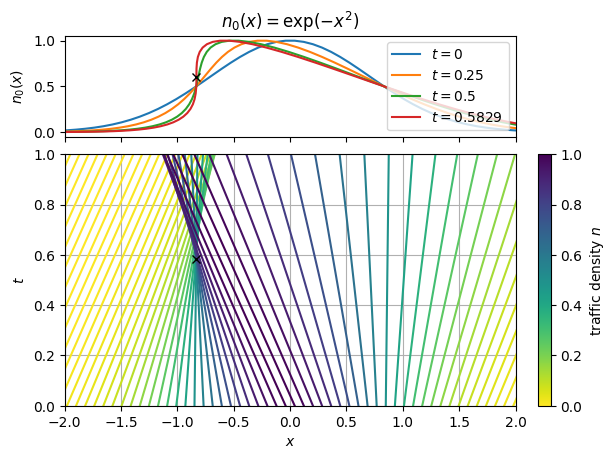
\[\begin{gather*} n_0(x) = e^{-x^2}, \qquad u(n) = 1-n, \qquad v_c(n) = 1-2n. \end{gather*}\]

../_images/c1c5025772a0020edb3bc4c9a7b53d21f21e0adc06c52a4f1627009629d9018d.png

This should make sense intuitively: when the density is high, the cars are slow, so the traffic from the left piles up, causing the density bump to move left. The buildup travels backward until a shockwave forms at about \(t\approx 0.58\). At this point, the characteristics intersect, and the analysis breaks down.

Do it! Can you figure out where an when the shock occurs in this case?

The shock forms when as soon as \(n_{,x}\) diverges. We can write the density at time \(t\) as

\[\begin{gather*} n(x, t) = n_0(x_0), \qquad x = x_0 + v\bigl(n_0(x_0)\bigr)t, \qquad v(n_0) = 1-2n_0. \end{gather*}\]

Holding \(t\) fixed and differentiating wrt \(x_0\), we have:

\[\begin{gather*} n_{,x}\d{x} = n_0'(x_0)\d{x_0}, \qquad \d{x} = \bigl(1 + v'(n_0)n_0'(x_0)t\bigr)\d{x_0}, \\ v'(n_0) = -2, \qquad n_0'(x_0) = -2x_0e^{-x_0^2}. \end{gather*}\]

Putting these together:

\[\begin{gather*} n_{,x} = n_0'(x_0)\diff{x_0}{x} = \frac{n_0'(x_0)}{1 - tn_0'(x_0)t}. = \frac{1}{\frac{1}{n_0'(x_0)} - 2t}. \end{gather*}\]

Hence, the shock forms first when

\[\begin{gather*} t = \frac{1}{2n_0'(x_0)} = \frac{-e^{x_0^2}}{4x_0}. \end{gather*}\]

Extremizing, we find the time at which the shock forms:

\[\begin{gather*} x_0 = \frac{1}{\pm\sqrt{2}}, \qquad t_{s} = \frac{\pm e^{1/2}}{2\sqrt{2}} = \pm 0.5829\cdots, \qquad n_0 = e^{-1/2} = 0.6065\cdots, \\ x_{s} = x_0 + (1-2n_0)t_{s} = \frac{\mp 1}{\sqrt{2}} \pm (1-2e^{-1/2})\frac{e^{1/2}}{2\sqrt{2}} = \mp \frac{4 - e^{1/2}}{2\sqrt{2}} = \mp 0.8313\cdots. \end{gather*}\]

The negative solution corresponds to the shock in the past that would have evolved into the gaussian at time \(t=0\).

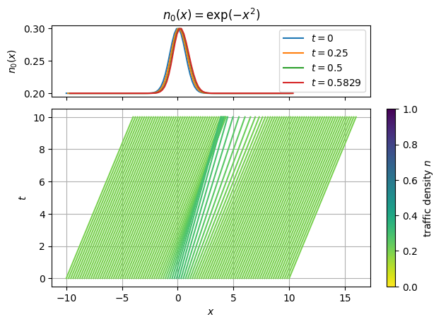
Trajectories#

Note that these characteristics do not represent the speed of the cars. Instead, they correspond to the “speed of sound” – the speed at which information passes through the traffic. To see what individual cars would do, we integrate the speed:

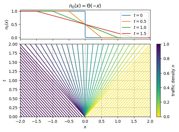
\[\begin{gather*} \dot{x}(t) = u\Bigl(n\bigl(x(t), t\bigr)\Bigr). \end{gather*}\]

Green-Light#

Another interesting case to consider is traffic stopped at a red light that turns green:

\[\begin{gather*} n(t=0) = \Theta(-x),\\ \end{gather*}\]

../_images/431f89bf637c4e2171349432c07b2ab988981ab991abc14e3aa892790b933cf6.png

To Do: Explore starting at green light.

Pick some reasonable values for \(n_{\max}\) and \(v_{\max}\) and check whether or not this model makes sense. How long does it take for a the \(n\)th car to start moving? What does the trajectory/speed of the \(n\)th car look like? If the light stays green for length of time \(T\) (what is a reasonable value?), how many cars get through?

Steady State and Stability#

One can do a perturbative analysis to figure out how quickly “sound waves” would flow through steady traffic in this model. Steady-state, constant-density flow occurs for any traffic density \(n\in[0,1]\). We now consider perturbing this solution

\[\begin{gather*} n(x, t) = n_0 + \delta(x, t)\\ \delta_{,t} + \underbrace{\Bigl(u(n_0) + n_0u'(n_0)\Bigr)}_{1-2n_0}\delta_{,x} + O(\delta^2) = 0. \end{gather*}\]

This is sometimes called “linearizing” the theory. This immediately admits the following plane-wave solution: \(\delta = e^{\I (kx-\omega t)}\):

\[\begin{gather*} \omega = (1-2n_0)k. \end{gather*}\]

We now have an interpretation of the characteristic velocity:

\[\begin{gather*} v_c = \frac{\omega}{k} = \omega'(k) = 1-2n_0. \end{gather*}\]

In the linearized theory this is both the phase and group velocity.

A Bump in the Road#

Here we play with a model of steady traffic flow, with a small bump introduced, slowing the traffic. Which direction does the shock propagate through the traffic?

../_images/336dd6b94a878cb96b1cd0488f1598c2939393472ded7a5c76590abb90fff5d7.png

Autonomous Vehicles#

To Explore: A Better Algorithm?

Suppose you are designing self-driving cars. It seems from these explorations and a little thought about characteristics that there is no good choice of model \(u(n)\) in the sense that – with the exception of starting from a red light – shocks will always form.

Some aspects of this model are not realistic – can you design something better that tends to smooth perturbations in the flow?

To start this exploration, let’s build a model for autonomous vehicles. To be physically reasonable, we will assume that the acceleration \(a = \ddot{x}\) of the vehicle is a function of the speed and positions of the other cars

\[\begin{gather*} \ddot{x}_i = f(\vect{x}, \dot{\vect{x}}). \end{gather*}\]

Realistically, we expect this to depend on only the following:

Current speed \(v=\dot{x}_i\). (Can be measured with the speedometer.)
Distance to car in front \(d = x_{i+1}-x_{i}\). (Can be measured with Lidar or parallax).
Relative speed of car in front \(s = \dot{x}_{i+1} - \dot{x}_{i}\). (Can be measured with doppler.)

One might also consider the following, but we neglect this for now:

Acceleration of the in front \(b = \ddot{x}_{i+1}\). (Can see the break lights.)

This is getting a little complex, so we introduce a class to keep things organized in our code.

from scipy.integrate import solve_ivp


class Units:
    """Some convenient units."""
    m = 1.0
    km = 1000 * m
    mile = 1609.344 * m

    s = 1.0
    h = 60 * 60 * s

    mph = mile / h

    n_max = 1 / (5 + 2) / m
    v_max = 70 * mile / h


u = Units()


class Cars:
    """A class to model a collection of autonomous vehicles.

    For definiteness, we model these on a ring of diameter L.
    """
    L = 1 * u.km
    a_max = 0.3 * 9.81 * u.m / u.s**2
    a_min = -9.81 * u.m / u.s**2
    v_max = 70 * u.mph
    n_max = 1 / (7 * u.m)

    x_unit, x_label = u.m, "m"
    t_unit, t_label = u.s, "s"

    def __init__(self, **kw):
        """Constructor just sets attributes, then calls init()."""
        for key in kw:
            if not hasattr(self, key):
                raise ValueError(f"Unknown {key=}")
            setattr(self, key, kw[key])
        self.init()

    def init(self):
        """Do any initialization here."""
        self.solve_ivp_args = dict(fun=self.compute_dy_dt,
                                   method='LSODA',
                                   atol=1e-4,
                                   rtol=1e-4)

    def get_dy_dt(self, x, v):
        """Return acclererations of each vehicle.
        
        This is a general function, but the default version here
        delegates to a simpler version.
        
        Arguments
        ---------
        x, v : array-like
            Velocity and position of cars.
        """
        # Check data:
        d = np.diff(x)
        assert np.all(np.diff(x)) > 0  # All cars in order.
        assert x[-1] - x[0] < self.L  # All carse on ring.

        # Add correct distance for last car
        d = np.concatenate([d, [x[0] + self.L - x[-1]]])
        s = np.concatenate([np.diff(v), [v[0] - v[-1]]])
        return self.get_a(v=v, d=d, s=s)

    def get_a(self, v, d, s):
        """Return the acceleration `a` from the following.
        
        Arguments
        ---------
        v : array
            Current speed.
        d : array
            Distance to car in front.
        s : array
            Relative speed of the care in front.
        """

        # Attempt to implement the first model
        n = 1 / d  # Density of cars
        u = self.v_max * (1 - n / self.n_max)

        # Accelerate to correct u as fast as possible.
        a = np.where(u < v, self.a_max, self.a_min)

        # Maybe more reasonable?
        # a = np.where(u < v, self.a_max * (v-u)/self.v_max, self.a_min)
        return a

    # The following are for solving the differential equations
    def pack(self, x, v):
        return np.ravel([x, v])

    def unpack(self, y):
        N_cars = len(y) // 2
        return np.reshape(y, (2, N_cars))

    def compute_dy_dt(self, t, y):
        x, v = self.unpack(y)
        a = self.get_dy_dt(x=x, v=v)
        return self.pack(v, a)

    def solve(self, x0, v0, dT=1 * u.s, **kw):
        """Evolve the cars by dT."""
        y0 = self.pack(x0, v0)
        t_span = (0, dT)
        kw = dict(self.solve_ivp_args, **kw)
        res = solve_ivp(y0=y0,
                        t_span=t_span,
                        **kw)
        assert res.success
        res.x, res.v = self.unpack(res.y[:, -1])
        return res

    def plot(self, x, v, ax=None):
        R = self.L / 2 / np.pi
        R_ = R / self.x_unit
        z_ = R_ * np.exp(1j * x / R)
        if ax is None:
            ax = plt.gca()
        th = np.linspace(0, 2 * np.pi, 300)
        ax.plot(R_ * np.cos(th), R_ * np.sin(th), '-k')
        ax.plot(z_.real, z_.imag, 'o', ms=10)
        ax.set(aspect=1,
               xlabel=f"$x$ [{self.x_label}]",
               ylabel=f"$y$ [{self.x_label}]")

Solving the PDE#

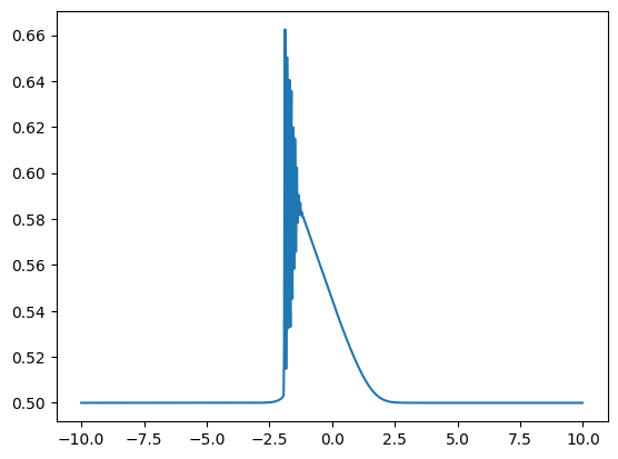
Here we try to solve the PDE… this does not work so well once shocks form!

%pylab
from scipy.integrate import solve_ivp

class Trafic:
    L = 20.0
    N = 256
    n0 = 0.5

    def __init__(self, **kw):
        for key in kw:
            if not hasattr(self, key):
                raise ValueError(f"Unknown {key=}")
            setattr(self, key, kw[key])
        self.init()
    
    def init(self):
        dx = self.L/self.N
        self.x = np.arange(self.N) * dx - self.L / 2
        self.ik = 2j*np.pi * np.fft.fftfreq(self.N, d=dx)
        self.solve_ivp_args = dict(
            fun=self.compute_dn_dt,
            method="LSODA",
            max_step=0.1,
        )
    
    def diff(self, f):
        return np.fft.ifft(self.ik*np.fft.fft(f)).real

    def diff(self, f):
        return np.gradient(f, self.x)
        
    def compute_dn_dt(self, t, n):
        return -self.diff(n*(1-n))
    
    def solve(self, n0, T):
        res = solve_ivp(y0=n0, t_span=(0, T), **self.solve_ivp_args)
        return res

m = Trafic(L=20.0, N=256*4)
n0 = np.where(m.x < 0, 0.5, 0.0)
n0[m.N//2] = 0.5
n0 = 0.5 + 0.1*np.exp(-m.x**2)
res = m.solve(n0, T=10)
plt.plot(m.x, res.y[:, -1])

Using matplotlib backend: inline
%pylab is deprecated, use %matplotlib inline and import the required libraries.
Populating the interactive namespace from numpy and matplotlib

[<matplotlib.lines.Line2D at 0x77dd3cf65150>]

../_images/30d11f7b3855018cbb30dc1f10d0924bbbcd899a4acdd828549bc308e669595d.png